This article was written by James Cancilla.
The STD2 operator is capable of performing online decomposition of a time series. More specifically, the STD2 operator is capable of ingesting a time series and decomposing it into seasonal, trend and residual components.
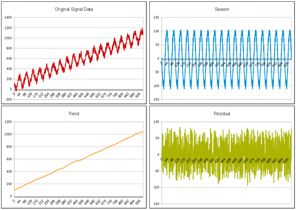
To better understand what these components mean, take a look at the following signal:

The above signal contains some very obvious characteristics. First, the data in the signal contains an oscillating pattern. In fact, this signal was created using a sine wave. This repeating cycle that you see in the signal is referred to as the season component. The second obvious characteristic is that the signal is continuously increasing. This is referred to as the trend component. Finally, there is obviously some randomness about the data. This randomness is referred to as the residual component.
By using this operator you can extract these three components into separate signals. The following image shows the result of decomposing the above signal using the STD2 operator.
The source code for this example can be found in the STD2Samples project on GitHub.
How It Works – Streaming Decomposition
The STD2 operator uses a common technique to decompose a time series into season, trend and residual components. The details of how this is done can be found in the paper listed in the References section below. Rather than reiterate the entire paper in this article, I am going to focus on one specific aspect of the decomposition technique, as it affects the data that is returned from the operator.
One of the first steps in the decomposition process is to smooth the time series. This helps to remove the random component from the signal and isolate the trend and cycle components. To perform this smoothing a technique called Centered Moving Average (CMA) is used. Here is an example of performing CMA on a time series:
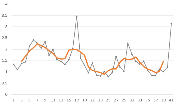
As you can see from the graph, the orange line is a smoothed representation of the original signal. However, the cost of performing this smoothing technique is that there will be data loss at the beginning and end of the smoothed signal. This is due to the fact that CMA requires a certain number of data points before and after the data point that is being averaged. In the above example, the average for the data point at t=3 was calculated by using the value of the data points at t=1, t=2, t=3, t=4 & t=5. The average could not be calculated for the data points at t=1 or t=2 since there were not enough preceding data points. Therefore, the smoothed times series does not have any values at t=1 or t=2.
This is an important point as this data loss will occur when using the STD2 operator. The STD2 operator uses a Centered Moving Average with a period equal to the length of a season (the length of a season is determined using the seasonLength parameter). As a result, the first half-season of data that is streamed into the operator will not return any results. If the input time series is continuous (in other words, the application will continue to run indefinitely), then all of the data points after the first half-season will generate output.
Analyzing Signal Segments
By default, the STD2 operator has a specially configured sliding window to handle a continuous stream of time series data. However, there may be cases where the data being analyzed are finite-length signals. In order to handle these types of signals, the operator can be configured with a tumbling window. When the window is flushed, the data in the window will be considered a finite-length time series and decomposition will occur only on that data. Since the time series is finite in length, the first and last half-season of data will not generate a result due to the use of the Centered Moving Average technique described in the previous section.
The STD2Samples project on GitHub contains an application called “STD2FiniteLength” that demonstrates how to decompose signal segments.
Operator Details
In this section you will find information about various important aspects of the STD2 operator. The complete documentation for the STD2 operator can be found on the STD2 Operator page in the Knowledge Center.
Parameters
The STD2 operator comes with a number of parameters. Details for each of the available parameters can be found on the STD2 Operator page. However, there are some important parameters that I want to highlight here.
- seasonLength – Specifies the length of a season. This is a required parameter.
- numSeasons – Specifies the number of seasons that should be ingested before performing the decomposition. The more seasons that are used when performing decomposition, the more accurate the results will be. The correct value to set will depend on the specific data. By default, this value is set to 2 since this is the minimum number of seasons that are required for the operator to work.
- trimNaNs – As explained in the previous sections, the STD2 operator will not return results for the first half-season of data (in the case of finite-length time series, results will also not be returned for the last half-season of data). If you still need tuples returned for the data that does not have results, set this value to false. By setting this value to false, tuples will be returned for all input data. For the first and last half-season of data, the season(), trend() and residual() output functions will return a value of NaN.
Inputs
The STD2 operator is capable of analyzing both a continuous stream of time series data and finite-length time series. Regardless of the the type of time series being analyzed, the inputTimeseries parameter must be set to an attribute on the input port with a type of float64
Outputs
There are three output functions that can be used to return the components of the signal. These output functions include:
- season() – Returns either a float64 or list<float64> that contains the season (or cycle) component.
- trend() – Returns either a float64 or list<float64> that contains the trend component.
- residual() – Returns either a float64 or list<float64> that contains the residual component.
Samples
The STD2Samples project on GitHub contains 4 applications that demonstrate how to use the STD2 operator. These applications are:
- STD2Basic – A simple example of how to ingest time series data from a file source and analyze it using the STD2 operator.
- STD2Random – Similar to the STD2Basic sample, however the data is randomly generated using a Custom operator. This can be helpful for tuning the STD2 operator with different types of input data.
- STD2FiniteLength – An example of how to configure a tumbling window to analyze signal segments
- STD2Anomaly – An example of how to use the STD2 operator in conjunction with the AnomalyDetector operator in order to perform anomaly detection on seasonal data.
References
#CloudPakforDataGroup