Implementing logistic regression from scratch in Python

Binary logistic regression is often mentioned in connection to classification tasks. The model is simple and one of the easy starters to learn about generating probabilities, classifying samples, and understanding gradient descent. This tutorial walks you through some mathematical equations and pairs them with practical examples in Python so that you can see exactly how to train your own custom binary logistic regression model.

Binary logistic regression explained

To understand and implement the algorithm, you must understand six equations, which I've explained below. I cautiously walk through them to give you the most intuition possible for how the algorithm works.

To perform a prediction, you use neural network-like notation; you have weights (w), inputs (x) and bias (b). You can iterate over an error and multiple them together and add the bias at the end like shown in the following example.

However, it's common to use vector notation. This means that w becomes a list of values (in Python terms). Vector notation enables you to use faster computation time, which can be highly beneficial if you want to do rapid prototyping with a larger data set. You write a list of values with bolder characters, for example, the vector w, and you can rewrite your equation above the following equation.

Furthermore, to get your prediction, you must use an activation function. In the case of binary logistic regression, it is called the sigmoid and is usually denoted by the Greek letter sigma. Another common notation is ŷ (y hat). In the following equation, you see the stable version of the sigmoid equation (Exp-normalize trick).

You can visualize the sigmoid function by the following graph.

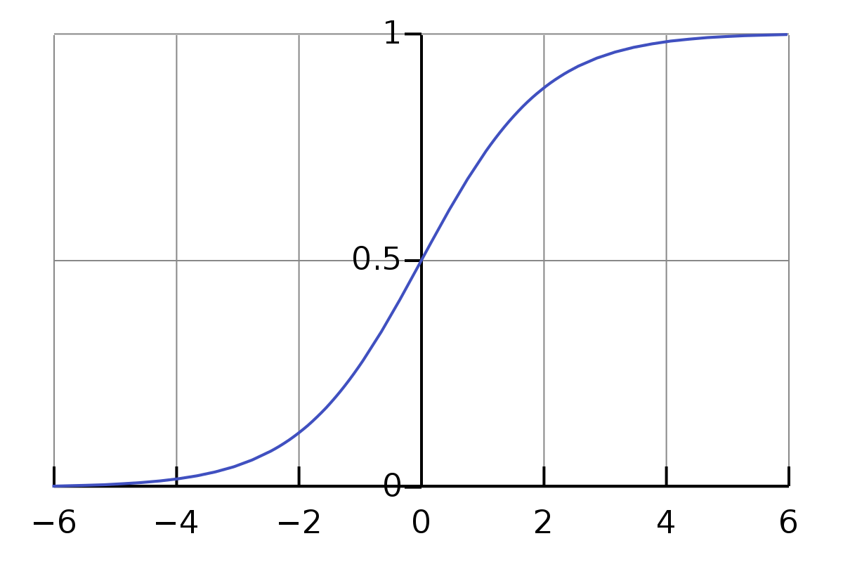
Sigmoid graph, showing how your input (x-axis) turns into an output in the range 0 - 1 (y-axis). From Wikipedia: Sigmoid function.

After you have the prediction, you can apply the basic gradient descent algorithm to optimize your model parameters, which are the weights and bias in this case. You do not use stochastic or mini-batch gradient descent in this article, but you can use the logistic regression section in the Speech and Language Processing article to see how these algorithms are implemented in a slightly different way.

The scary part for beginners is the unknown parameters and Greek letters, so the following list gives explanations.

• θ (theta) is the parameter. For example, your weights or bias.
• θ_t is the current value of the parameter.
• θ_t+1 is the next value of the parameter.
• η (eta) is the learning rate, which is usually set to a value between 0.1 and 0.0001.
• ∇L refers to the gradients (∇, nabla) of the (L)oss function, which I introduce below. It takes in your inputs (x), your parameter values (θ), and the labels (y).

The loss function (also known as a cost function) is a function that is used to measure how much your prediction differs from the labels. Binary cross entropy is the function that is used in this article for the binary logistic regression algorithm, which yields the error value.

Looking at the plus sign in the equation, if y = 0, then the left side is equal to 0, and if y = 1, then the right side is equal to 0. Effectively, this is how you measure how much your prediction ŷ differs from label y, which can only be 0 or 1 in a binary classification algorithm.

Now, to calculate the gradients to optimize your weights using gradient descent, you must calculate the derivative of your loss function. In other words, you must calculate the partial derivative of binary cross entropy. You can compactly describe the derivative of the loss function as seen as follows; for a derivation, see Section 5.10 in the Speech and Language Processing article.

When you have the final values from your derivative calculation, you can use it in the gradient descent equation and update the weights and bias.

Seeing all of these equations can be scary, especially if you do not have formal education. The best way to learn is by applying the equations, which is why I'll apply a practical example in Python with the help of NumPy for numerical computations.

Python example

The first thing in a Python example is to choose your data set. You need it to be a binary classification data set, so I chose one from the scikit-learn library that is called the "Breast Cancer Wisconsin" data set. You get several features that you can use to determine whether a person has breast cancer. Read more about the UCI, Breast Cancer Wisconsin data set.

To load the data set, I created a small piece of code to get the data into training and testing sets in Pandas DataFrames.

import pandas as pd
from sklearn.model_selection import train_test_split
from sklearn.datasets import load_breast_cancer

def sklearn_to_df(data_loader):
    X_data = data_loader.data
    X_columns = data_loader.feature_names
    x = pd.DataFrame(X_data, columns=X_columns)

    y_data = data_loader.target
    y = pd.Series(y_data, name='target')

    return x, y

x, y = sklearn_to_df(load_breast_cancer())

x_train, x_test, y_train, y_test = train_test_split(
    x, y, test_size=0.2, random_state=42)

Afterward, you import all of the data, libraries, and models that you need for the training part. As seen below, you'll come back to the scikit-learn logistic regression model and compare it to your custom implementation at the end. You start by creating your custom model and using the fit methods with your training data for 150 iterations (epochs).

from sklearn.metrics import accuracy_score
from sklearn.linear_model import LogisticRegression
from logistic_regression import LogisticRegression as CustomLogisticRegression
from data import x_train, x_test, y_train, y_test

lr = CustomLogisticRegression()
lr.fit(x_train, y_train, epochs=150)

Now, I will dive deep into the fit method that handles the entire training cycle. There are many things to unpack, but you should notice that you use the math from the prior explanation on binary logistic regression.

First, you take in the input and do a small transformation that is not covered in this article. You can see the full details in the GitHub repository for this article.

Next, you explain all of the functions seen in the fit method below after the walkthrough of the fit method. You start by doing the weight and sigmoid calculation. As you saw in the explanation, you must multiply the inputs with the weights and add the bias. Then, you input these weights into the sigmoid function and get predictions.

Then comes the part where you must think about gradient descent. You can compute the loss by the implemented compute_loss function and the derivative by the compute_gradients function. The loss is not used in the model (only the derivative of the loss is used), but you can monitor the loss to determine when your model cannot learn more, which is how the 150 epochs were chosen for the model. Finally, you update the parameters of the model, and then you start the next iteration and continue iterating until you reach 150 iterations.

def fit(self, x, y, epochs):
    x = self._transform_x(x)
    y = self._transform_y(y)

    self.weights = np.zeros(x.shape[1])
    self.bias = 0

    for i in range(epochs):
        x_dot_weights = np.matmul(self.weights, x.transpose()) + self.bias
        pred = self._sigmoid(x_dot_weights)
        loss = self.compute_loss(y, pred)
        error_w, error_b = self.compute_gradients(x, y, pred)
        self.update_model_parameters(error_w, error_b)

        pred_to_class = [1 if p > 0.5 else 0 for p in pred]
        self.train_accuracies.append(accuracy_score(y, pred_to_class))
        self.losses.append(loss)

To implement the stable version of the sigmoid function, you just had to implement the equation and run through every value. This is not done as a vector calculation like you saw when you multiplied the weights by the inputs. This is due to the if-else statement that makes sure that no errors happen when the output of the sigmoid is negative or positive infinity. See more details in the Exp-normalize trick.

def _sigmoid(self, x):
    return np.array([self._sigmoid_function(value) for value in x])

def _sigmoid_function(self, x):
    if x >= 0:
        z = np.exp(-x)
        return 1 / (1 + z)
    else:
        z = np.exp(x)
        return z / (1 + z)

This is the loss function that is implemented as a vectorized solution exactly like you saw in the explanation section. You are essentially finding all of the errors by comparing your ground truth y_true to your predictions y_pred (also known as y hat from your explanation section).

def compute_loss(self, y_true, y_pred):
    # binary cross entropy
    y_zero_loss = y_true * np.log(y_pred + 1e-9)
    y_one_loss = (1-y_true) * np.log(1 - y_pred + 1e-9)
    return -np.mean(y_zero_loss + y_one_loss)

Now, you get to calculate the gradients, which are what you use to update the model parameters. The equations look complicated if you are new to math, but the following implementation is not too complicated. You start by finding the difference (how much your model predicted wrong) and use it to calculate the gradients for the bias by finding the average error.

Afterward, as you saw in the explanation section, you simply have to multiply the difference by the inputs (x). Then, you need to find the average of each gradient, which is simple in Python. Now, you can return the changes and update your model.

def compute_gradients(self, x, y_true, y_pred):
    # derivative of binary cross entropy
    difference =  y_pred - y_true
    gradient_b = np.mean(difference)
    gradients_w = np.matmul(x.transpose(), difference)
    gradients_w = np.array([np.mean(grad) for grad in gradients_w])

    return gradients_w, gradient_b

Perhaps the least complicated part of the gradient descent algorithm is the update. You have already calculated the errors (gradients), and now you just have to update the weights for the next iteration so that the model can learn from the next errors.

def update_model_parameters(self, error_w, error_b):
    self.weights = self.weights - 0.1 * error_w
    self.bias = self.bias - 0.1 * error_b

After fitting over 150 epochs, you can use the predict function and generate an accuracy score from your custom logistic regression model.

pred = lr.predict(x_test)
accuracy = accuracy_score(y_test, pred)
print(accuracy)

You find that you get an accuracy score of 92.98% with your custom model. The following code shows how to do the prediction, which is a repetition of the code in the fit function. The extra addition is that you threshold and classify anything with a probability lower than 0.5 as class 0 (not breast cancer) and anything higher than 0.5 as class 1 (breast cancer).

def predict(self, x):
    x_dot_weights = np.matmul(x, self.weights.transpose()) + self.bias
    probabilities = self._sigmoid(x_dot_weights)
    return [1 if p > 0.5 else 0 for p in probabilities]

After getting your accuracy score, you compare with the logistic regression model from the scikit-learn library by using the methods that are implemented in their library. I named the methods the same in the custom implementation for easy reference.

model = LogisticRegression(solver='newton-cg', max_iter=150)
model.fit(x_train, y_train)
pred2 = model.predict(x_test)
accuracy2 = accuracy_score(y_test, pred2)
print(accuracy2)

You find that the accuracy is almost equal, with scikit-learn being slightly better at an accuracy of 95.61%, beating your custom logistic regression model by 2.63%.

Conclusion

In this article, you learned how to implement your custom binary logistic regression model in Python while understanding the underlying math. You saw how similar the logistic regression model can be to a simple neural network.