Article
Implementing a virtual rail architecture
New architecture maximizes both throughput and redundancyOn 16 December, 2024, IBM announced our cluster network for NVIDIA accelerated computing. In that announcement, we mentioned a "rail-like" architecture built on top of a leaf/spine network, and a "Virtual Rail Redundancy technique" to provide both the throughput of an AI reference network and the redundancy of a cloud-based leaf/spine network.
IBM’s multi-tenant AI training network enables our customers to push massive bandwidth through. When we compared the AI workload times of this new architecture against our on-prem Infiniband-based training cluster, both clusters were within 1-5% of each other, even though the latter always beat the former in specific benchmarks.
Further, the redundancy was thoroughly tested very early in the build. Our first customer is IBM watsonx; they’ve been able to run large, continuous jobs while we’ve performed necessary maintenance on the network.
In this article, we'll show you Nvidia’s reference rail-optimized AI network cluster architecture and explain how we developed the Virtual Rail architecture. It assumes a basic knowledge of leaf/spine network architectures as well as simple networking principles.
Cloud network primer
IBM’s cloud network architecture makes use of a fairly generic leaf/spine layout. This document won’t get into the details of that; please refer to the previous link. But from a high level, that architecture and our internal software defined network (SDN) provides the cloud servers with full path redundancy as well as the necessary throughput to handle the cloud workloads. The entire network including the servers uses the Border Gateway Protocol (BGP) for routing and equal cost multi-pathing (ECMP) for load balancing. Finally, the network is built assuming a certain over-subscription rate, as it’s not financially feasible or realistic to expect a 1:1 subscription rate.
GPU and AI network architecture
A typical network architecture for GPU-driven AI workloads is normally different from the aforementioned highly redundant cloud network. This section provides a high-level description of the reference architecture most often used for on-prem deployments and discusses why that doesn't apply well to multi-tenant cloud workloads, where redundancy is still key.
Reference: Rail architecture
Nvidia has published a reference-optimized architecture that uses Infiniband instead of Ethernet. However, the same principles apply to their Ethernet version. Each server has a series of eight single-port 400GigEth NICs like the one shown in figure 1, which align internally to the eight GPUs in it. Each 400GigEth port is connected to one of eight upstream leaf or rail switches, as shown in figure 2.

Figure 1: Single-port Nvidia Connect-X 7 NIC (source: FS.com)

Figure 2: A server with 8 400GigEth NICs
Those eight rail switches are then uplinked to one of 16 upstream TOR-based spines, each by the 2x400GigEth. The results are 32 uplink and 32 downlink 400GigEth ports, which allow for 32 hosts total in that small cluster of eight rail switches, and all while maintaining a 1:1 subscription rate. And because the spines have 64x400GigEth ports on them, it allows for four clusters of 32 hosts, or 128 hosts total, as shown in figure 3.

Figure 3: 128 hosts in a rail network
Benefits
Latency
One important benefit is a consistently low overall network latency. TOR-based switches typically have a much lower latency than chassis-based switches. And in this design, the packets never traverse a chassis, so the latency numbers can be kept low.
But as we'll see, consistent latency is actually more important than low latency, although low latency still matters.
Throughput and bandwidth
Another key aspect of this design is literally no oversubscription. Each rail switch in figure 2 has exactly 32x400GigEth inbound from servers and 32x400GigEth outbound to the spines. This subscription rate and bandwidth is important enough as a requirement that it must be retained even with a redundant cloud design for the same workloads.
If specific AI workloads can be contained to 32 hosts on the same set of eight rail switches, it provides a further benefit of even lower latency and lack of ECMP at the source rail switch egress to the spines and spine egress back to the target rail switch.
Concerns
Redundancy
Network path redundancy is a major area of concern. Although the servers have eight uplinks to their respective rail switches, if one of those switches fails, the Nvidia libraries used on the hosts haven't been coded to shift that load to one of the other uplinks. Instead, the job may crash if an uplink or rail switch fails.
The cost of a crash could be wasted hours, days, weeks, or even months, depending on the training job and the last time a checkpoint dump was done. For a purely on-prem private cluster, this lack of network path redundancy is probably fine. But for a multi-tenant public or private cloud where customers could be inside the company as well as outside of it, this lack of redundancy and reliability isn’t acceptable.
Cluster size limitations
The cluster size in this architecture is limited to 128 nodes. It can be expanded by using a second layer of spines attached to the first, creating clusters of spines as shown in figure 4.
This requires removing one of the 32-node clusters so that the spines have uplink ports to connect to a new SuperSpine layer while retaining a 1:1 subscription rate within that cluster. It also means that between the clusters of spines, a 1:1 subscription will be impossible.
To retain full performance in this sort of expanded architecture, you’ll want to keep training jobs within a specific 16-spine cluster. This architecture is challenging to use for a multi-tenant cluster due to job placement requirements.

Figure 4: A larger TOR-based rail with SuperSpines
Multi-tenant GPU/AI network architecture
We'll now combine the input from the previous two sections to produce a single, cohesive, fully redundant and performant network architecture. We'll start with the server NICs, then look at the leaf nodes, and, most importantly, we'll wrap up with the chassis spines.
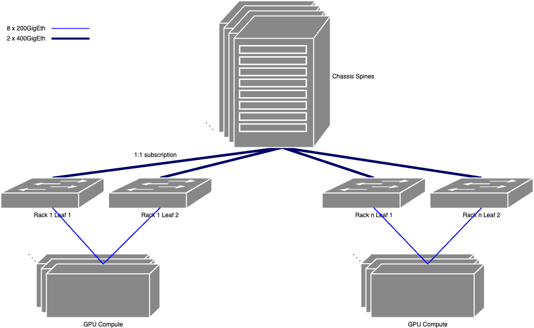
Figure 5: GPU leaf/spine architecture with chassis
Servers and NICs
Figure 5 illustrates the style of leaf/spine network that we built, using chassis-based switches as spines. We'll refer to it throughout the rest of this article.
We'll start at the servers and NICs and move up to the spines. In Figure 5 we have three servers per rack. However, any number of servers that data center can provide power and cooling for is applicable here.
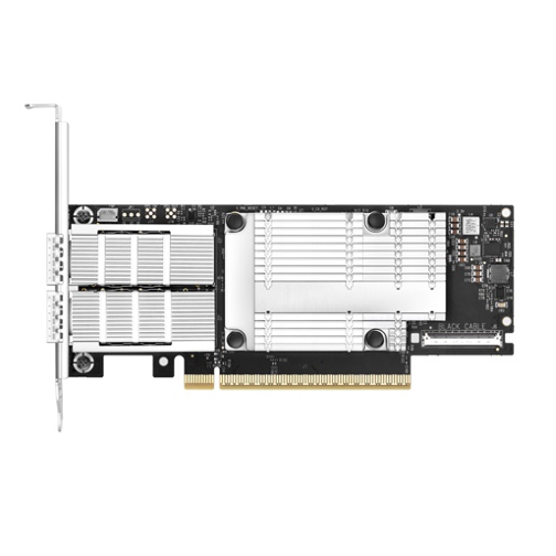
Figure 6: Dual-port Nvidia ConnectX-7 NIC (source: FS.com)
The servers aren’t equipped with 8x400GigEth NICs, but rather eight 2x200G NICs like the one shown in figure 6. Each NIC is still capable of 400Gbps throughput in total, but each has two ports on it instead of one. This one change has a huge ripple effect upwards and throughout the entire architecture. The primary purpose for this change is port-level redundancy at each NIC.
As with our cloud servers, the redundancy and traffic direction is handled by our SDN. BGP is used to announce specific IP addresses for each NIC. A given IP address (for example, 10.11.12.1/32) is announced out of NIC1:port 1 and NIC1:port 2. The next IP address (for example, 10.11.12.2/32) is announced out of NIC2:port 1 and NIC2:port 2. This sequence repeats until there are a series of eight /32 IP addresses announced from each server, one per NIC.
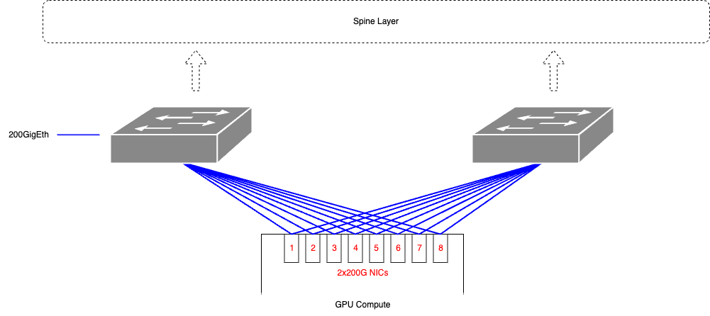
Figure 7: A server with eight 2x200GigEth NICs
Figure 7 shows how a server with eight 2x200GigE NICs connects upstream to the two leaf switches in the rack. Through BGP, each NIC announces its specific /32 IP address to both of the TORs, which provides the server redundant ingress.
To keep the server's routing table minimized, it's only listening for the default (0.0.0.0/0) route in BGP. We also use specific NIC and SDN tuning to make sure that the host, using the NIC, sends half of the queue-pairs (QPs) out the first port, and half out the second.
Leaf switches
Like in the cloud architecture, there are two leaf switches in each rack. These are much higher bandwidth than is used in a typical cloud infrastructure: all ports would be 400GigEth-capable.
The uplink and downlink counts have to be managed carefully to retain a 1:1 subscription rate. Because the hosts are connected using 200GigEth, two host connections would count towards one uplink at 400GigEth.
Referring to figure 5 and the six upstream spines (which we'll discuss shortly), along with the aforementioned three servers, we have the following requirements:
- 3 hosts at 8x200Gig each, or 4.8Tbps
- 6 spines requiring a total of 4.8Tbps leaf throughput or 800Gpbs per leaf per spine
- 2x400GigEth per leaf per spine
This means that each leaf uplinks to each spine with two connections, or 2x400GigEth.
Dynamic load balancing: Improving outbound throughput
Because of the six spines, each leaf switch has a total 12x400GigEth uplinks. BGP uses the usual ECMP method to determine which egress port to send a new flow towards the upstream spine switches. ECMP usually uses the input Ethernet port:source IP:source port:destination IP:destination port tuple to spread new flows evenly across outbound ports. This works exceptionally well when there are thousands of potential source and destination hosts throughout the network.
With AI clusters, those source and destination numbers drop significantly. The unfortunate and real result is that the switch will often overload several of the uplink interfaces while leaving others under-utilized or not utilized at all. Entropy is needed to keep the links properly balanced, and when you have elephant flows with AI workloads, the entropy just isn't there.
Broadcom's Dynamic Load Balancing (DLB) is one solution for this challenge. DLB is available on their newer Trident and Tomahawk ASICs. What it attempts to do is look at actual, real-time port utilization after flows have been assigned to their respective egress ports. Very quickly, the ASIC will determine if ports are under- or potentially over-utilized, and, when appropriate, shift specific flows from one egress port to another.
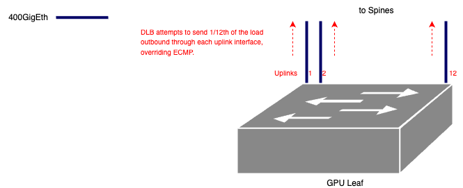
Figure 8: DLB attempts to improve outbound throughput
Figure 8 shows our leaf switch with its 12 uplinks. DLB will do an excellent job at splitting the load to a near perfect 1/12th of the total for each uplink, which is much better than standard ECMP can do on its own.
The challenge with DLB is that it's not available on the ASICs used in the chassis switches. This will provide a huge challenge for the spine throughput, which we'll look at in the next section.
RoCEv2
The leaves are configured to cooperate with the SDN on the hosts to provide an RDMA over converged Ethernet network path between the GPU compute hosts. We won't include details of our RoCE configuration in this article; we did collaborate closely with our network vendor Arista to properly test our configurations.
Spines
Similar to the cloud network, this architecture features a set of spines at the top. Those spines can be scaled from four to six to however many are necessary for throughput and rack count. The line cards in these chassis-based switches are all 400GigEth in this case, versus the 100GigEth in the previous leaf/spine.
There's a throughput problem when introducing spines and ECMP into the mix, however, and that's what we'll focus on from this point. One simple metric we used while pursuing this challenge was the link utilization of the 200GigE link at the destination leaf switch, towards the GPU host. Prior to any of the virtual rail design, we were seeing a consistent utilization of 138Gbits/sec on a 200GigE link. After the design was put in place, 180Gbits/sec on a 200GigE link, or a 30% improvement!
| Spine Configuration | Dest Leaf 200GigE Port Utilization |
|---|---|
| No Rails | 138 Gbps |
| Rails | 180 Gbps |
ECMP challenges
We had to meet two specific challenges, both a result of relying on BGP's ECMP:
- Unbalanced queue-pairs (QP)
- Unbalanced Ethernet port utilization
Unbalanced queue-pairs
Let's take a look at rack-to-rack communication. Our example source NIC's IP address will be 10.11.12.1/32, and the NIC in the destination host in another rack has the IP of 10.11.12.25/32. Figure 9 depicts an ideal spread for the outbound QP traffic from the host on the left, and inbound to the host on the right, if we're assuming eight QPs, or four and four.
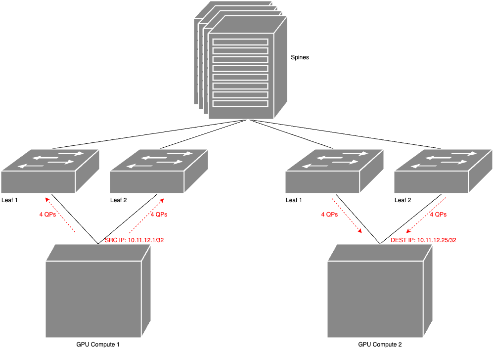
Figure 9: Ideal distribution of outbound and inbound QPs
Unfortunately, with the spine layer utilizing standard BGP ECMP, that balance is rarely achieved. It means the interfaces on the NIC on the destination server were either under-utilized or over-utilized, the latter causing congestion notifications (CNs) resulting in a performance hit.
The reason is shown in figure 10. An incoming flow from the source rack is sent using ECMP across one of the four available links from that spine towards the destination rack. The spine has no understanding of the QPs involved and whether a flow should go outbound towards leaf 1 or leaf 2. It'll select one of those links and pin that flow to it.

Figure 10: Spine using ECMP to select an outbound link for the destination IP
In our example, the result is that there was always an unbalanced distribution of QPs at the destination host. Figure 11 shows what that looked like with three QPs landing on the NIC's first port, and the remaining five landing on the second port. Because of the size of these flows, it meant that the five QPs hitting the second port overwhelmed that NIC's available bandwidth, resulting in CNs and a performance degradation.

Figure 11: QPs on destination side not balanced
Unbalanced Ethernet port utilization
Because of the ECMP at the spine layer, the link utilization problem at the host is also present at the leaf layer, specifically between the destination leaves and the spines. This problem is associated with the relatively low number of overall flows transiting the spines. As discussed previously, low entropy is a challenge for ECMP to retain a near-perfect balance of outbound traffic towards a destination.
At IBM, from the spine's perspective, we would sometimes see an unbalanced load distribution on the four destination links (two per downstream leaf). Examples would include an outbound load distribution of 10%, 50%, 0%, 40%. Results like this are not ideal. If the spines had a technology like DLB available to them, that link utilization would be far more equal. But the QP problem would likely still exist to a lesser extent. A different solution is needed.
Creating the virtual rail
Through further collaboration with Arista, we came up with a solution that deploys virtual rails, or paths, on the spine layer. This is considerably different from the whole concept of a traditional leaf/spine network architecture, specifically because it involves the spine in decision-making for the network flows versus having it act as a "dumb" layer-3 routing switch. It does mean that the spines' configuration complexity will increase—in some cases by quite a bit.
Two rails for the QPs
If we refer back to Figure 12 and the unbalanced QPs, it might make sense at first to use two rails: one for the first switch in the rack, one for the second. And that does work, too. The QPs balance out on the destination how, but the overall traffic throughput only increases by maybe 10%. The reason is that each rail has multiple outbound downlinks that the spine still has to use ECMP. It’s an improvement, but we decided to push it further.
Multiple rails: One per downlink
We can improve the previous two-rail setup by adding more of them. Specifically, we used one rail per link between each spine and a rack. If we look at a single spine and count the number of downlinks from it to any given rack (for example, 4, or 6, or so on), that's the total number of rails we configured on that spine.

Figure 12: One rail per downlink
Figure 12 shows an example where there are four total downlinks from any given spine to any rack, based on the required throughput needed. In this case, we create four rails on each spine.
Again, like the previous rail solution, this was performed on each spine by first defining the rails, then applying them to the appropriate downlink ports for each leaf switch, and then moving the BGP peering for those interfaces into the respective rails.
What this solution does is solve for both our challenges: it keeps the QPs aligned, and it completely removes any and all ECMP from the spines. A packet that enters a rail from a source leaf switch will only ever have exactly one outbound port to egress towards the destination leaf.
Redundancy
Remember that the server’s routing table is minimized to a default route, meaning it will always send traffic towards the leaf that’s advertising the route regardless of what happens in another rack. Further, the rails on the spines literally prevent any cross-talking by removing all ECMP. This means that a failed switch in a destination rack will cause leaf switches in the source rack to black-hole traffic.
To solve this, we configured the rails to selectively share routes between them. This, again, happened at the spine layer. The goal was to ensure that the routes known in one half of the rails are also known in the other, and vice versa.
In fact, the leak formula is fairly simple. We can assume TotalRails describes the total number of rails on the spine, CurrentRail is the rail we’re configuring for leaking, and TargetRail is the rail that the current rail will leak to. At the spine and for the odd number leaf switches in each rack (for example, leaf1), the leak formula looks like the following:
TargetRail == CurrentRail + (TotalRails/2)
So, for example, if we're working on the leaking from Rail 1, and we have four rails in total, then the rail to leak to would be:
TargetRail == 1 + (4/2)
TargetRail == 3
Rail 1's routes would be leaked to Rail 3, and vice versa for the even number (for example, leaf2) switches in each rack. The formula looks like this:
TargetRail == CurrentRail - (TotalRails/2)
Again, we take Rail 3 as our source rail since it's associated with leaf2 in each rack. The rail that we'd leak Rail 3's routes to is:
TargetRail == 3 - (4/2)
TargetRail == 1

Figure 13: Leaf in destination rack fails
Figure 13 shows this in a simple diagram. We can see that the first leaf switch in the destination rack has failed or is down for maintenance. Because of the route leaks, the first leaf in every source rack will still be able to send traffic to that destination rack. This happens because, at the spines, the packets are leaked into the rails of the second leaf switch in that rack. The traffic will arrive but at a slower rate; this allows the AI workloads to continue if at a slower pace while the network is repaired.
Summary
The well-known leaf/spine network architecture is heavily used and prized by cloud-scale organizations throughout the industry, given its excellent throughput, redundancy, and reliability. Newer, faster rail-optimized networks are appearing for on-prem AI workloads that don't lend themselves as well to multi-tenant infrastructures. In this article, we've shown that the leaf/spine architecture, with some additional configurations, can hit near-Infiniband rail-optimized network performance while retaining the redundancy and reliability needed for multi-tenancy.
Next steps
Interested in learning more about scaling efficiently with on-demand access to NVIDIA GPUs? Check out NVIDIA GPU Instances.
Acknowledgements
The author would like to thank the following for their considerable contributions to both the architecture and this document:
- Kiran Pillai – Distinguished Engineer, IBM Cloud Networking
- Eran Gampel – Distinguished Engineer, IBM Cloud Networking
- Drew Thorstensen – Senior Technical Staff Member, IBM Cloud Compute
- Bengi Karacali-Akyamac – Senior Research Scientist, IBM Research
- Seetharami Seelam – Distinguished Engineer, IBM Research
- Matt Newsom – Technical Lead, Systems Engineering, Arista Networks
- Sudhakaran Subramanian – Technical Lead, Systems Engineering, Arista Networks