Classifying data using the SVM algorithm using R on watsonx.ai

Support vector machines (SVMs) are robust supervised machine learning algorithms for classification and regression tasks. They are grounded in mathematical concepts like linear algebra, optimization theory, and hyperplanes.

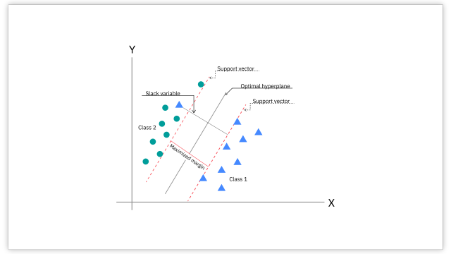
SVMs are supervised learning techniques that specialize in dividing data into classes by creating a hyperplane with maximum margin between the classes. A hyperplane divides a space of a higher dimension into two parts, such as a line dividing a 2 dimensional plane or a plane dividing a 3 dimensional space. The number of dimensions in the space will correspond to the number of attributes, or features of the data inputted when fitting the model.

During classification, SVMs work by solving quadratic optimization problems. In this process, they identify the most effective hyperplane using the data points closest to the decision boundary, which separates the spaces corresponding to the different classes. SVMs are inherently limited to binary classification, however a combination of SVMs can be used to create a multi-class classifier. This versatility renders SVMs suitable for both binary and multi-class classification problems.

SVMs can be applied to Gaussian, multinomial, and logistic regression to predict continuous values by finding a hyperplane that depicts the overall pattern of the data. Linear SVM, a variant, employs linear regression to determine the hyperplane that maximizes the margin between classes for efficient classification.

SVMs can handle linear and nonlinear tasks. For nonlinear issues, SVMs transform the original data into higher-dimensional spaces using kernel functions, such as linear, polynomial, radial basis function (RBF), or sigmoid kernels. The choice of kernel and hyperparameters depends on the use case and data characteristics, but it significantly influences the SVM model's performance. Therefore, it is essential to understand the underlying concepts and fine-tune these parameters for successful SVM implementation. In R, techniques like cross-validation and grid search are commonly used for parameter tuning.

SVMs are more effective in high-dimensional spaces and cases where the number of dimensions exceeds the number of samples. They find application in various real-world scenarios, such as text and hypertext categorization, classification of images, bioinformatics, protein fold and remote homology detection, handwriting recognition, and remote sensing. SVMs are also more easily interpretable than other machine learning algorithms, which lends itself well to use cases where decision justification is important.

SVMs can be computationally expensive for large data sets, and are thus undesirable if training time is an important factor in these cases. SVMs are also sensitive to feature scaling, meaning that extra pre-processing to normalize or standardize features is necessary to ensure that accurate decision boundaries are drawn. Finally, SVMs are not suitable for use cases where probability estimates are needed for predictions.

In this tutorial, we implement an SVM on the popular Iris data set and provide a step-by-step beginner's guide to implementing SVMs in R programming. We'll cover all the key steps, from data exploration to evaluation, and provide a solid foundation for implementing SVMs.

A Jupyter notebook containing the R code samples used in this tutorial are available in this GitHub repo for you to download and import into your watsonx project.

Prerequisites

• Create an IBM Cloud account

Steps

Step 1: Set up your environment

While you can choose from several tools, this tutorial walks you through how to set up an IBM account to use a Jupyter Notebook. Jupyter Notebooks are widely used within data science to combine code, text, images, and data visualizations to formulate a well-formed analysis.

1. Log in to watsonx.ai using your IBM Cloud account.

2. Create a watsonx.ai project.

3. Create a Jupyter Notebook.

From here, a notebook environment opens for you to load your data set and copy code from this beginner tutorial to tackle a simple classification problem.

Step 2: Install and load the required library

In this step, we'll install the e1071 library, a crucial package for SVM implementation in R.

#Install the required package
install.packages("e1071")
install.packages('caret')

#Load the required library
library("e1071")
library("caret")

Step 3: Load the Iris data set

Next, we'll load the built-in Iris data set, making it accessible for analysis and modeling tasks in the R environment.

#Load the Iris data set
data(iris)

Step 4: Explore the data set

In this crucial step, we will delve into the Iris data set and understand its characteristics, including its structure, summary statistics, and variable types. This exploratory data analysis will provide foundational insights for subsequent analysis, data manipulation, and modeling, guiding informed decisions on the most suitable techniques and models.

#Explore the Iris data set
head(iris)
summary(iris)
str(iris)

The following screen capture shows an overview of the Iris data set.

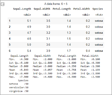
The data set consists of 150 rows, with 50 samples for each of the three iris species: setosa, versicolor, and virginica. Here, each row represents an observation or a data point.

The data set has five columns: sepal length, sepal width, petal length, petal width, and species. The notations <dbl> and <fct> denote the data types associated with the columns. <dbl> represents a column with numeric, double-precision (decimal) data type. In statistical terms, it typically indicates a continuous or numerical variable. On the other hand, <fct> denotes a column with categorical or factor data type. Factors in R take on a limited and fixed set of values, such as categories or labels.

Now, let's associate these data types with one of the columns, say sepal length (Sepal.Length (Numeric, )).

• Min., Max.: The statistical summary provides insights into the distribution of sepal lengths, with the minimum value at 4.300 and the maximum value at 7.900. This information indicates the range of sepal lengths in the data set.
• 1st Qu. (25th percentile): The value 5.100 denotes the lower quartile, below which 25% of the sepal lengths are distributed.
• Median: The median value of 5.800 indicates the midpoint of the sepal lengths, providing a central tendency measure that is less influenced by extreme values.
• Mean: The mean value of 5.843 represents the average sepal length.
• 3rd Qu. (75th percentile): The value 6.400 indicates the upper quartile, below which 75% of the sepal lengths fall.

Similar interpretations can be made for other numeric columns like Sepal.Width, Petal.Length, and Petal.Width.

As for <fct>, it represents the categorical column, species, which has three categories: setosa, versicolor, and virginica. For this column, the statistics include the count of each category. For instance, there are 50 observations corresponding to each species.

Step 5: Create training and testing subsets

In this step, we will split the Iris data set into training and testing subsets to facilitate model training and evaluation. The model learns from training data and is tested on unseen data, ensuring it can generalize well to new instances. This process helps assess the model's generalization capabilities and mitigates the risk of overfitting.

In this tutorial, we'll randomly split the data set into 70% training and 30% testing sets.

set.seed(123)
trainIndex <- sample(1:nrow(iris), 0.7 * nrow(iris))
iris_train <- iris[trainIndex, ]
iris_test <- iris[-trainIndex, ]

Step 6: Explore the data set through plots and graphs

Visualization is a crucial aspect of data exploration as it provides a deeper understanding of the relationships within a data set. In this step, we will use visualizations to explore the Iris data set and extract meaningful insights. We aim to discern patterns, distributions, and potential separations among the different iris species based on their sepal length and width. This visual inspection will allow us to identify potential challenges, such as class overlaps and distinct separations, which will aid in selecting an appropriate SVM kernel and parameter settings.

#Visualize the Iris data set
#Plot sepal length vs. sepal width with species as color and point type
plot(iris$Sepal.Length, iris$Sepal.Width, col = iris$Species, pch = 19, main = "Sepal Length vs Sepal Width", xlab = "Sepal Length", ylab = "Sepal Width")

#Add legend
legend("topright", legend = levels(iris$Species), col = unique(iris$Species), pch = 19, title = "Species")

The following shows the output of visualizing the iris data set in a plot.

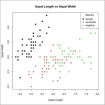
Let's interpret the distribution of points for each species:

• setosa: The spread of the black dots on the left side of the plot indicates the characteristic sepal dimensions for Iris setosa, whose flowers generally have shorter and broader sepals.
• versicolor: The spread of the pink dots across the middle of the plot indicates that Iris versicolor flowers exhibit a moderate range of sepal lengths and widths, positioning them between the setosa and virginica species.
• virginica: The dispersion of the green dots toward the right side of the plot indicates that Iris virginica flowers typically possess longer sepals and exhibit a moderate range of sepal widths.

The insights obtained from this visualization will guide subsequent decisions in the SVM modeling process, enhancing the overall effectiveness of the SVM classifier. For instance, distinct separations between species in the scatterplot may suggest the effectiveness of a linear kernel, while overlapping clusters may indicate the suitability of a nonlinear kernel.

The data in the iris data set has 4 dimensions along with the classification, but we have only visualized the relationship between 2 of the data’s dimensions and the classification. We encourage you to make more 2 dimensional plots comparing different features of the flowers to understand more about the data.

Step 7: Train the SVM model

Training an SVM model is pivotal in machine learning workflows, especially for classification tasks. In this step, we will train the SVM model using the training subset. We will use the svm function from the e1071 library and configure the model with a linear kernel and carefully chosen parameters.

SVMs typically work by identifying an optimal decision boundary that maximally separates distinct classes in the feature space. Here, the choice of a linear kernel indicates that the model intends to establish a linear decision boundary to distinguish between different iris species.

#Train the SVM model classifier
model <- svm(Species ~ ., data = iris_train, kernel = "linear", cost = 0.1, scale = TRUE)

The trained SVM model will be evaluated using the testing subset to gauge its predictive accuracy.

Step 8: Fine-tune the parameters of the SVM model

Parameter tuning involves improving model accuracy based on the insights gained during evaluation. This iterative process helps identify the optimal combination that minimizes errors, maximizes accuracy, and mitigates overfitting or underfitting.

In this step, we will refine the performance of our SVM model by fine-tuning its parameters. We will use the tune function with the svm algorithm while exploring various combinations of the epsilon (ε) and cost hyperparameters. Epsilon is a hyperparameter in the SVM algorithm that controls the margin width. In contrast, cost, another crucial hyperparameter, determines the penalty for misclassifying a datapoint or being within the margin width of the separating hyperplane. The goal is to find the combination of epsilon and cost values that result in the darkest shade on the color gradient, indicating optimal hyperparameter settings for the SVM model.

#Tune the SVM model's parameters
set.seed(123)
tuned_model <- tune(svm, Species ~ ., data = iris, ranges = list(epsilon = seq(0, 1, 0.1), cost = 2^(2:7)))
plot(tuned_model)

The following graph is a parameter optimization plot of the tuned SVM model.

In this optimization plot, the color gradient, which transitions from dark to light violet, indicates the performance of the SVM model based on the combination of epsilon and cost. Darker shades represent better-performing models, while lighter shades represent less optimal models. The specific values on the X and Y axes indicate the different combinations of hyperparameter values tested during the tuning process.

Step 9: Evaluate the SVM model

Model evaluation is crucial in machine learning, as it offers insights into how well the trained model generalizes to new, unseen data. The evaluation process involves making predictions on the testing subset and comparing them with the actual values, allowing us to quantify the model's accuracy and identify potential areas for improvement.

In this step, we will evaluate the model using the testing subset and generate a confusion matrix for detailed analysis. The confusion matrix will indicate the classification accuracy of the SVM model.

#Evaluate the SVM prediction model
predicted <- predict(model, iris_test[, -5])
confusionMatrix(table(predicted, iris_test$Species))

The following graph shows the confusion matrix for the SVM model.

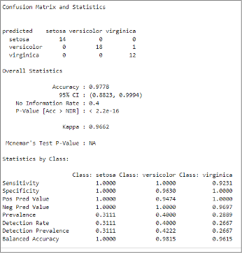
The confusion matrix section depicts the instances of accurate classification and misclassification by the SVM model. The three rows in the confusion matrix correspond to the actual classes in the dataset: setosa, versicolor, and virginica. Conversely, the three columns represent the classes predicted by the SVM model. The numbers in the confusion matrix represent the count of instances for each combination of actual and predicted classes.

Let's interpret the results of the confusion matrix and statistics:

• Confusion matrix

  • For the actual "setosa" class

    • Fourteen instances were correctly predicted as "setosa" (true positives).
    • Zero instances were incorrectly predicted as "versicolor."
    • Zero instances were incorrectly predicted as "virginica."

  • For the actual "versicolor" class

    • Eighteen instances were correctly predicted as "versicolor" (true positives)
    • Zero instances were incorrectly predicted as "setosa."
    • One instance was incorrectly predicted as "virginica."

  • For the actual "virginica" class

    • Twelve instances were correctly predicted as "virginica" (true positives).
    • Zero instances were misclassified as "setosa."
    • Zero instances were misclassified as "versicolor."

• Overall statistics

  • Accuracy: The SVM model accurately classified 44 of 45 samples. So, the overall accuracy of the model is 97.78%.
  • 95% confidence interval (CI): The CI provides a range estimate for the true accuracy of the model, which is between 88.23% and 99.94%.
  • No information rate (NIR): NIR is the accuracy achieved by always predicting the majority class, which is 40%.
  • P-value: The P-value assesses whether the model's accuracy differs significantly from the NIR. Here, the extremely low P-value (nearly zero) strongly suggests that the model's accuracy significantly surpasses what could be achieved by merely predicting the majority class, indicating the model's effectiveness.
  • Kappa: The Kappa statistic measures the agreement between predicted and actual classifications. Here, a value of 0.9662 indicates high agreement.
  • McNemar's test P-value: The McNemar's test assesses if there is a significant difference in performance between two related classifiers. Here, "NA" suggests that the test might not be applicable or was not performed.

• Statistics by class Let's explore the metrics for one class, say, setosa.

  • Sensitivity (true positive rate): This metric represents the model's accuracy in identifying actual positive instances. Here, 1.0000 indicates perfect identification of all setosa flowers among actual setosa instances.
  • Specificity (true negative rate): This metric indicates the model's accuracy in predicting actual negative instances. Here, 1.0000 indicates that the model correctly identified all instances that are not setosa among actual non-setosa instances.
  • Positive predictive value (precision): This metric reflects the accuracy of predicted positives that are true positives. Here, 1.0000 signifies 100% correctness when predicting setosa instances.
  • Negative predictive value: This metric indicates the accuracy of predicted negatives that are true negatives. Here, 1.0000 indicates 100% correctness when predicting non-setosa instances.
  • Prevalence: This metric indicates the proportion of the dataset belonging to the specific class. The proportion of actual setosa instances in the data set is 0.3111.
  • Detection rate: This metric indicates the proportion of instances correctly identified by the model. Here, the model correctly identifies 31.11% of actual setosa instances.
  • Detection prevalence: This metric represents the proportion of predicted positive instances. Among the instances predicted as setosa, 31.11% are actual setosa instances.
  • Balanced accuracy: This statistic indicates the average sensitivity and specificity, providing an overall performance measure. For setosa, 1.0000 indicates a perfectly balanced performance.

To summarize the results, the confusion matrix and detailed statistics provided a comprehensive understanding of the model's strengths and potential areas for improvement. The SVM model demonstrated excellent performance with high accuracy and balanced metrics for all three classes. Sensitivity, specificity, and positive predictive values were all notably high.

Following this evaluation, you may adjust specific parameters, such as the kernel type, cost, and epsilon. This fine-tuning allows experimentation with different SVM configurations to enhance the model's capabilities.

Summary and next steps

In this tutorial, you learned that SVMs are powerful supervised learning tools applicable to classification and regression tasks. You explored the steps to implement SVM in R using IBM Watson Studio Jupyter Notebooks on watsonx.ai.

You were taken through a comprehensive journey, from initial data exploration to evaluation. You first split the dataset into training and testing subsets. Then, you visually explored the dataset using a scatterplot to identify potential challenges, such as class overlaps and distinct separations. You then trained the SVM model and refined the model's performance by fine-tuning various combinations of the epsilon (ε) and cost hyperparameters. Finally, you evaluated the SVM model. From the confusion matrix statistics, you observed that the SVM model demonstrated high accuracy and balanced metrics across all three classes: setosa, versicolor, and virginica. The insights gained from the confusion matrix will guide further model refinement, contributing to an iterative and improvement-focused machine-learning process.

Try watsonx for free

Build an artificial intelligence (AI) strategy for your business on one collaborative AI and data platform called IBM watsonx, which combines new generative AI capabilities powered by foundation models and traditional machine learning into a powerful platform spanning the AI lifecycle. With watsonx.ai, you can train, validate, tune, and deploy models with ease and build AI applications in a fraction of the time with a fraction of the data.

Try watsonx.ai, the next-generation studio for AI builders. Explore more articles and tutorials about watsonx on IBM Developer.