Create a confusion matrix with R

A confusion matrix (or error matrix) is a visualization method for classifier algorithm results. More specifically, a confusion matrix is a table that breaks down the number of ground truth instances of a specific class against the number of predicted class instances. Confusion matrices are one of several evaluation metrics that are used to measure the performance of a classification model in machine learning. They can be used to calculate a number of other model performance metrics, such as precision and recall, among others.

Confusion matrices can be used with any classifier algorithm, such as Naïve Bayes, logistic regression models, and decision trees. Because of their wide applicability in data science and machine learning models, many packages and libraries come preloaded with functions for creating confusion matrices, such as R's caret package.

In this tutorial, we’ll use a number of R packages to walk through creating a confusion matrix for a simple binary classification problem. We will also cover how to compute classifier metrics, such as precision and F1 score. This tutorial focuses on creating confusion matrices with R programming. If you want to learn how to produce confusion matrices in Python, you may check out our confusion matrix Python tutorial.

Confusion matrix layout

In a confusion matrix, columns represent the predicted values of a given class while rows represent the actual values (that is, ground truth) of a given class, or vice-versa. Note that the reverse also appears in research. This grid structure is a convenient tool for visualizing model classification accuracy by displaying the number of correct predictions and incorrect predictions for all classes alongside one another.

A standard confusion matrix template for a binary classifier is divided into four quadrants:

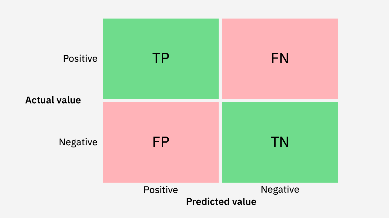
The top-left box provides the number of true positives (TP), being the number of correct predictions for the positive class. The box beneath it is false positives (FP), those negative-class instances incorrectly identified as positive cases. These are called type I errors in statistics. The top-right box is the number of false negatives (FN), the actual positive instances erroneously predicted negative. Finally, the bottom-right box displays the number of true negatives (TN), which are actual negative class instances accurately predicted as negative. Totaling up each of these values provides the model’s total number of predictions.

Prerequisites

You need an IBM Cloud account to create a watsonx.ai project.

Steps

Step 1. Set up your environment

While you can choose from several tools, this tutorial walks you through how to set up an IBM account to use a Jupyter Notebook. Jupyter Notebooks are widely used within data science to combine code, text, images, and data visualizations to formulate a well-formed analysis.

1. Log in to watsonx.ai using your IBM Cloud account.

2. Create a watsonx.ai project.

3. Create a Jupyter Notebook

A notebook environment opens for you to load your data set and copy code from this tutorial to tackle a simple data visualization task. To view how each block of code works, each step’s code block is best inserted as a separate cell of code in your watsonx.ai project notebook.

Step 2. Install and import relevant libraries

You'll need a few libraries for this tutorial. Make sure to import the required packages. If they're not installed, you can install them with the following code:

install.packages("cvms", repos = "https://cloud.r-project.org")
install.packages("caret", repos = "https://cloud.r-project.org")
install.packages("ggplot2", repos = "https://cloud.r-project.org")
install.packages("dplyr", repos = "https://cloud.r-project.org")
install.packages("ConfusionTableR", repos = "https://cloud.r-project.org")

You can check whether the packages are successfully installed by running the following three commands. If the following three lines are reprinted in your terminal output, all necessary libraries have been succesfully installed.

library(cvms)
library(caret)
library(ggplot2)
library(dplyr)
library(ConfusionTableR)

Step 3. Load the data

For this tutorial, we will not load data from an outside repository. The confusion matrix is a data visualization tool for evaluating classification algorithm performance. As such, our data will be the actual and predicted values for a classification task. The actual values (or, ground truth) are the manually created class labels for a dataset. The predicted values are the predicted class labels for that same dataset.

The ground truth and predicted values used for this tutorial are:

# load list of original dataset values
gt_pt1 <- c(0, 0, 0, 0, 0, 0, 0, 0, 1, 1, 1, 0, 0, 0, 0, 0, 1, 0, 0, 0, 0, 0, 0, 0, 0, 0, 0, 0, 0, 1, 0, 0, 0, 0, 1, 1, 0, 0, 0, 0, 0, 0, 0, 0, 0, 0, 0, 0, 0, 0, 0, 0, 0, 0, 0, 0, 0, 0, 0, 0, 0, 1, 1, 0, 0, 0, 1, 0, 0, 0, 0, 0, 0, 0, 0, 0, 0, 0, 0, 0, 0, 0, 0, 0, 0, 0, 0, 1, 0, 1, 0, 0, 0, 0, 0, 0, 0, 0, 1, 0, 0, 0, 0, 1, 0, 0, 0, 0, 0, 0, 0, 0, 0, 0, 0, 0, 1, 0, 0, 0, 1, 0, 1, 0, 0, 0, 0, 0, 0, 0, 0, 0, 0, 0, 0, 0, 0, 0, 0, 1, 0, 0, 0, 1, 0, 0, 0, 0, 0, 0, 0, 0, 0, 0, 0, 0, 0, 0, 0, 0, 1, 0, 0, 0, 0, 0, 0, 0, 0, 0, 0, 0, 0, 0, 1, 0, 0, 1, 0, 0, 0, 0, 0, 0, 0, 0, 0, 0, 0, 0, 0, 0, 0, 0, 0, 1, 0, 1, 0, 0, 1, 0, 0, 0, 0, 0, 0, 0, 0, 0, 0, 1, 0, 0, 1, 0, 0, 0, 0, 0, 1, 0, 0, 0, 0, 0, 0, 0, 1, 0, 0, 0, 0, 0, 0, 0, 1, 0, 0, 1, 0, 0, 0, 1, 0, 0, 0, 0, 0, 0, 0, 0, 0, 0, 0, 1, 0, 0, 0, 0, 0, 0, 0, 0, 0, 0, 0, 0, 0, 0, 0, 0, 1, 1, 0, 0, 0, 0, 0, 0, 0, 0, 0, 0, 0, 0, 0, 0, 0, 0, 1, 0, 0, 0, 0, 0, 0, 0, 0, 0, 0, 0, 0, 0, 0, 0, 0, 0, 1, 0, 1, 0, 0, 0, 0, 0, 0, 0, 0, 0, 0, 1, 0, 0, 0, 0, 0, 0, 0, 0, 0, 0, 0, 1, 0, 0, 0, 0, 0, 0, 0, 0, 0, 0, 0, 0, 0, 0, 0, 0, 1, 0, 1, 0, 0, 0, 0, 0, 0, 0, 0, 0, 0, 0, 0, 0, 0, 1, 0, 0, 0, 0, 1, 0, 0, 0, 0, 0, 0, 0, 0, 1, 1, 0, 0, 0, 0, 0, 0, 0, 0, 0, 0, 0, 0, 0, 0, 0, 0, 0, 0, 1, 0, 0, 0, 1, 0, 0, 0, 0, 0, 0, 0, 0, 0, 0, 0, 0, 0, 0, 0, 0, 0, 0, 0, 0, 0, 0, 0, 0, 0, 0, 0, 0, 0, 0, 0, 0, 0, 0, 1, 0, 0, 0, 0, 0, 0, 1, 0, 0, 0, 0, 0, 1, 0, 0, 0, 1, 0, 0, 1, 0, 0, 0, 0, 1, 0, 0, 0, 0, 0, 0, 0, 0, 0, 0, 0, 0, 0, 1, 0, 0, 0, 0, 0, 0, 0, 1, 0, 0, 0, 0, 0, 0, 0, 0, 0, 0, 0, 0, 0, 1, 1, 0, 0, 0, 0, 0, 0, 0, 0, 0, 0, 0, 0, 0, 0, 0, 0, 0, 0, 0, 1, 1, 0, 0, 1, 0, 1, 0, 0, 0, 0, 0, 1, 0, 0, 0, 0, 1, 0, 0, 1, 0, 0, 1, 0, 0, 0, 0, 0, 0, 0, 0, 0, 0, 1, 0, 0, 0, 1, 0, 0, 0, 0, 0, 1, 0, 0, 0, 0, 1, 0, 0, 0, 0, 0, 0, 0, 0, 0, 0, 0, 0, 1, 1, 1, 0, 0, 0, 0, 0, 0, 0, 0, 0, 0, 1, 0, 0, 1, 0, 1, 0, 0, 0, 0, 0, 0, 0, 0, 0, 0, 0, 0, 0, 0, 0, 0, 0, 0, 0, 0, 0, 0, 0, 0, 1, 0, 0, 0, 0, 0, 1, 0, 0, 0, 0, 0, 0, 0, 0, 0, 0, 0, 0, 0, 0, 0, 0, 0, 0, 0, 0, 0, 0, 0, 0, 0, 0, 0, 0, 0, 1, 0)

gt_pt2 <- c(0, 0, 0, 0, 0, 0, 0, 0, 0, 0, 0, 0, 0, 0, 0, 0, 0, 0, 0, 0, 0, 0, 0, 0, 0, 1, 0, 0, 0, 0, 0, 0, 0, 0, 1, 0, 0, 1, 0, 0, 0, 1, 0, 0, 0, 0, 0, 0, 0, 0, 1, 1, 1, 0, 0, 0, 0, 1, 0, 1, 0, 1, 0, 0, 0, 0, 0, 0, 0, 0, 0, 0, 0, 0, 0, 0, 0, 0, 0, 0, 1, 0, 1, 0, 0, 1, 0, 1, 0, 0, 0, 0, 0, 0, 1, 1, 0, 1, 0, 0, 0, 0, 0, 0, 0, 0, 0, 0, 0, 0, 1, 0, 0, 0, 0, 0, 0, 0, 0, 0, 0, 0, 0, 0, 0, 0, 0, 0, 1, 1, 0, 0, 1, 0, 1, 0, 0, 1, 0, 1, 0, 0, 0, 0, 0, 0, 0, 0, 0, 1, 0, 0, 0, 0, 0, 0, 0, 0, 1, 0, 1, 0, 0, 0, 0, 0, 0, 0, 0, 0, 0, 0, 0, 0, 0, 0, 0, 0, 0, 0, 0, 0, 0, 0, 0, 1, 1, 0, 0, 0, 0, 1, 1, 0, 0, 0, 0, 0, 0, 0, 0, 1, 0, 0, 0, 0, 0, 0, 1, 1, 0, 0, 0, 0, 0, 1, 0, 0, 0, 0, 0, 1, 0, 0, 1, 0, 1, 0, 1, 0, 0, 0, 0, 0, 0, 0, 0, 0, 0, 0, 0, 0, 0, 0, 0, 0, 0, 0, 1, 0, 1, 0, 0, 0, 0, 0, 0, 0, 0, 0, 0, 0, 0, 0, 0, 0, 0, 0, 1, 0, 0, 0, 0, 0, 1, 0, 0, 0, 0, 1, 0, 0, 0, 0, 0, 0, 0, 0, 0, 0, 0, 0, 1, 1, 0, 0, 0, 0, 0, 0, 0, 1, 0, 0, 1, 0, 0, 0, 0, 0, 0, 1, 0, 0, 0, 0, 0, 1, 1, 0, 0, 0, 0, 0, 0, 1, 1, 1, 0, 0, 0, 0, 0, 0, 0, 0, 0, 0, 0, 0, 0, 0, 1, 0, 0, 0, 0, 0, 0, 0, 0, 1, 1, 0, 1, 0, 0, 0, 0, 0, 0, 0, 1, 0, 0, 0, 0, 0, 0, 0, 0, 0, 0, 1, 0, 0, 0, 0, 0, 0, 0, 0, 0, 0, 0, 0, 0, 0, 0, 0, 0, 0, 0, 0, 1, 0, 0, 0, 0, 0, 0, 0, 0, 0, 0, 0, 0, 0, 1, 0, 0, 0, 0, 1, 0, 0, 0, 0, 0, 0, 0, 0, 0, 0, 0, 0, 0, 0, 0, 0, 0, 0, 0, 0, 0, 1, 0, 0, 1, 0, 0, 0, 0, 1, 0, 0, 0, 0, 0, 0, 0, 0, 1, 0, 0, 1, 0, 0, 0, 1, 1, 0, 0, 0, 0, 1, 0, 0, 0, 0, 0, 1, 0, 0, 1, 0, 0, 0, 0, 1, 0, 0, 0, 0, 0, 0, 0, 1, 0, 0, 0, 0, 0, 0, 0, 0, 0, 0, 0, 0, 0, 0, 1, 0, 0, 0, 0, 0, 0, 0, 0, 0, 0, 0, 0, 0, 0, 0, 0, 0, 0, 0, 0, 0, 0, 0, 0, 0, 0, 0, 0, 0, 0, 0, 0, 0, 0, 0, 0, 0, 0, 0, 0, 0, 0, 0, 0, 0, 0, 1, 0, 0, 0, 0, 0, 0, 0, 0, 0, 0, 0, 0, 0, 1, 0, 0, 1, 0, 0, 0, 0, 0, 0, 0, 0, 0, 0, 0, 0, 0, 0, 0, 0, 1, 0, 1, 0, 0, 0, 0, 0, 0, 0, 0, 0, 0, 0, 0, 0, 0, 0, 0, 0, 0, 0, 0, 0, 1, 0, 0, 0, 0, 1, 0, 0, 0, 1, 0, 0, 0, 0, 0, 0, 0, 0, 0, 1, 1, 0, 0, 0, 0, 0, 0, 0, 0, 0, 0, 1, 0, 1, 0, 0, 0, 0, 0, 0, 0, 1, 1, 0, 0, 0, 0, 0, 0, 0, 0, 0, 1, 0)

gt_pt3 <- c(0, 1, 0, 0, 0, 0, 1, 0, 0, 0, 0, 1, 0, 0, 0, 0, 0, 1, 0, 0, 0, 0, 1, 0, 0, 0, 0, 0, 0, 0, 0, 0, 0, 0, 0, 0, 0, 0, 0, 0, 0, 0, 0, 1, 0, 0, 0, 0, 0, 0, 0, 0, 0, 0, 1, 0, 0, 0, 0, 0, 1, 0, 0, 0, 0, 0, 0, 0, 0, 0, 0, 0, 1, 0, 0, 0, 0, 0, 0, 0, 0, 0, 0, 0, 1, 0, 0, 0, 0, 0, 0, 0, 0, 0, 0, 0, 0, 0, 0, 0, 1, 0, 1, 0, 0, 0, 1, 0, 0, 0, 1, 0, 0, 0, 0, 0, 0, 0, 0, 0, 0, 1, 0, 0, 0, 0, 0, 0, 0, 0, 0, 0, 0, 0, 0, 0, 0, 0, 0, 0, 0, 0, 0, 0, 0, 0, 0, 0, 0, 0, 0, 1, 0, 0, 0, 0, 0, 0, 0, 0, 0, 0, 0, 0, 0, 1, 0, 0, 0, 0, 0, 0, 0, 1, 0, 0, 0, 1, 0, 0, 0, 0, 0, 0, 0, 0, 0, 0, 0, 1, 0, 1, 1, 1, 1, 1, 0, 0, 0, 0, 0, 0, 0, 0, 0, 0, 0, 0, 0, 0, 1, 1, 0, 0, 1, 0, 1, 0, 0, 0, 0, 1, 0, 0, 1)

ground_truth <- c(gt_pt1, gt_pt2, gt_pt3)

# load list of model output prediction values
preds_pt1 <- c(0, 0, 0, 0, 0, 0, 0, 0, 1, 1, 1, 0, 0, 0, 0, 0, 1, 0, 0, 0, 0, 0, 0, 0, 0, 0, 0, 0, 0, 1, 0, 0, 0, 0, 1, 1, 0, 0, 0, 0, 0, 0, 0, 0, 0, 0, 0, 0, 0, 0, 0, 0, 0, 0, 0, 0, 0, 0, 0, 0, 0, 1, 1, 0, 0, 0, 1, 0, 0, 0, 0, 0, 0, 0, 0, 0, 0, 0, 0, 0, 0, 0, 0, 0, 0, 0, 0, 0, 0, 1, 0, 0, 0, 0, 0, 0, 0, 0, 1, 0, 0, 0, 0, 1, 0, 0, 0, 0, 0, 0, 0, 0, 0, 0, 0, 0, 1, 0, 0, 0, 1, 0, 1, 0, 0, 0, 0, 0, 0, 0, 0, 0, 0, 0, 0, 0, 0, 0, 0, 0, 0, 0, 0, 1, 0, 0, 0, 0, 0, 0, 0, 0, 0, 0, 0, 0, 0, 0, 0, 0, 1, 0, 0, 0, 0, 0, 0, 0, 0, 0, 0, 0, 0, 0, 1, 0, 0, 1, 0, 0, 0, 0, 0, 0, 0, 0, 0, 0, 0, 0, 0, 0, 0, 0, 0, 1, 0, 1, 0, 0, 1, 0, 0, 0, 0, 0, 0, 0, 0, 0, 0, 1, 0, 0, 1, 0, 0, 0, 0, 0, 0, 0, 0, 0, 0, 0, 0, 0, 1, 0, 0, 0, 0, 0, 0, 0, 1, 0, 0, 1, 0, 0, 0, 0, 0, 0, 0, 0, 0, 0, 0, 0, 0, 0, 0, 1, 0, 0, 0, 0, 0, 0, 0, 0, 0, 0, 0, 0, 0, 0, 0, 0, 1, 1, 0, 0, 0, 0, 0, 0, 0, 0, 0, 0, 0, 0, 0, 0, 0, 0, 1, 0, 0, 0, 0, 0, 0, 0, 0, 0, 0, 0, 0, 0, 0, 0, 0, 0, 1, 0, 1, 0, 0, 0, 0, 0, 0, 0, 0, 0, 0, 1, 0, 0, 0, 0, 0, 0, 0, 0, 0, 0, 0, 0, 0, 0, 0, 0, 0, 0, 0, 0, 0, 0, 0, 0, 0, 0, 0, 0, 1, 0, 1, 0, 0, 0, 0, 0, 0, 0, 0, 0, 0, 0, 0, 0, 0, 0, 0, 0, 1, 0, 1, 0, 0, 0, 0, 0, 0, 0, 0, 1, 0, 0, 0, 0, 0, 0, 0, 0, 0, 0, 0, 0, 0, 0, 0, 0, 0, 0, 0, 1, 0, 0, 0, 1, 0, 0, 0, 0, 0, 0, 0, 0, 0, 0, 0, 0, 0, 0, 0, 0, 0, 0, 0, 0, 0, 0, 0, 0, 0, 0, 0, 0, 0, 0, 0, 0, 0, 0, 0, 0, 0, 0, 0, 0, 0, 1, 0, 0, 0, 0, 0, 1, 0, 0, 0, 1, 0, 0, 1, 0, 0, 0, 0, 1, 0, 0, 0, 0, 0, 0, 0, 0, 0, 0, 0, 0, 0, 1, 0, 0, 0, 0, 0, 0, 0, 0, 0, 0, 0, 0, 0, 0, 0, 0, 0, 0, 0, 0, 0, 1, 1, 0, 0, 0, 0, 0, 0, 0, 0, 0, 0, 0, 0, 0, 0, 0, 0, 0, 0, 0, 0, 1, 0, 0, 1, 0, 0, 0, 0, 0, 0, 0, 0, 0, 0, 0, 0, 1, 0, 0, 1, 0, 0, 1, 0, 0, 0, 0, 0, 0, 0, 0, 0, 0, 1, 0, 0, 0, 1, 0, 0, 0, 0, 0, 1, 0, 0, 0, 0, 0, 0, 0, 0, 0, 0, 0, 0, 0, 0, 0, 0, 0, 0, 1, 0, 0, 0, 0, 0, 0, 0, 0, 0, 0, 0, 1, 0, 0, 0, 0, 0, 0, 0, 0, 0, 0, 0, 0, 0, 0, 0, 0, 0, 0, 0, 0, 0, 0, 0, 0, 0, 0, 0, 0, 0, 0, 0, 0, 0, 0, 0, 1, 0, 0, 0, 0, 0, 0, 0, 0, 0, 0, 0, 0, 0, 0, 0, 0, 0, 0, 0, 0, 0)

preds_pt2 <- c(0, 0, 0, 0, 0, 0, 0, 0, 1, 0, 0, 0, 0, 0, 0, 0, 0, 0, 0, 0, 0, 0, 0, 0, 0, 0, 0, 0, 0, 0, 0, 0, 0, 0, 0, 1, 0, 0, 0, 0, 0, 0, 0, 0, 1, 0, 0, 1, 0, 0, 0, 1, 0, 0, 0, 0, 0, 0, 0, 0, 1, 1, 0, 0, 0, 0, 0, 0, 0, 0, 0, 0, 0, 0, 0, 0, 0, 0, 0, 0, 0, 0, 0, 0, 0, 0, 0, 0, 0, 0, 1, 0, 1, 0, 0, 1, 0, 0, 0, 0, 0, 0, 0, 0, 1, 1, 0, 1, 0, 0, 0, 0, 0, 0, 0, 0, 0, 0, 0, 0, 0, 0, 0, 0, 0, 0, 0, 0, 0, 0, 0, 0, 0, 0, 0, 0, 0, 0, 1, 1, 0, 0, 1, 0, 1, 0, 0, 1, 0, 1, 0, 0, 0, 0, 0, 0, 0, 0, 0, 1, 0, 0, 0, 0, 0, 0, 0, 0, 1, 0, 0, 0, 0, 0, 0, 0, 0, 0, 0, 0, 0, 0, 0, 0, 0, 0, 0, 0, 0, 0, 0, 0, 0, 0, 0, 0, 0, 0, 0, 0, 0, 1, 1, 0, 0, 0, 0, 0, 0, 0, 0, 0, 0, 0, 0, 0, 0, 0, 1, 1, 0, 0, 0, 0, 0, 0, 0, 0, 0, 0, 0, 1, 0, 0, 1, 0, 0, 0, 1, 0, 0, 0, 0, 0, 0, 0, 0, 0, 0, 0, 0, 0, 0, 0, 0, 0, 0, 0, 0, 0, 0, 0, 0, 0, 0, 0, 0, 0, 0, 0, 0, 0, 0, 0, 0, 0, 0, 0, 1, 0, 0, 0, 0, 0, 0, 0, 0, 0, 0, 1, 0, 0, 0, 0, 0, 0, 0, 0, 0, 0, 0, 0, 0, 0, 0, 0, 0, 0, 0, 0, 0, 1, 0, 0, 0, 0, 0, 0, 0, 0, 0, 1, 0, 0, 0, 0, 0, 1, 1, 0, 0, 0, 0, 0, 0, 1, 0, 1, 0, 0, 0, 0, 0, 0, 0, 0, 0, 0, 0, 0, 0, 0, 1, 0, 0, 0, 0, 0, 0, 0, 0, 1, 1, 0, 1, 0, 0, 0, 0, 0, 0, 0, 0, 0, 0, 0, 0, 0, 0, 0, 0, 0, 0, 0, 0, 0, 0, 0, 0, 0, 0, 0, 0, 0, 0, 0, 0, 0, 0, 0, 0, 0, 0, 0, 1, 0, 0, 0, 0, 0, 0, 0, 0, 0, 0, 0, 0, 0, 1, 0, 0, 0, 0, 1, 0, 0, 0, 0, 0, 0, 0, 0, 0, 0, 0, 0, 0, 0, 0, 0, 0, 0, 0, 0, 0, 1, 0, 0, 1, 0, 0, 0, 0, 1, 0, 0, 0, 0, 0, 0, 0, 0, 0, 0, 0, 1, 0, 0, 0, 1, 1, 0, 0, 0, 0, 1, 0, 0, 0, 0, 0, 1, 0, 0, 1, 0, 0, 0, 0, 1, 0, 0, 0, 0, 0, 0, 0, 0, 0, 0, 0, 0, 0, 0, 0, 0, 0, 0, 0, 0, 0, 0, 0, 0, 0, 0, 0, 0, 0, 0, 0, 0, 0, 0, 0, 0, 0, 0, 0, 0, 0, 0, 0, 0, 0, 0, 0, 0, 0, 0, 0, 0, 0, 0, 0, 0, 0, 0, 0, 0, 0, 0, 0, 0, 0, 0, 0, 0, 0, 1, 0, 0, 0, 0, 0, 0, 0, 0, 0, 0, 0, 0, 0, 0, 0, 0, 1, 0, 0, 0, 0, 0, 0, 0, 0, 0, 0, 0, 0, 0, 0, 0, 0, 0, 0, 0, 0, 0, 0, 0, 0, 0, 0, 0, 0, 0, 0, 0, 0, 0, 0, 0, 0, 0, 0, 0, 0, 0, 0, 0, 0, 0, 1, 0, 0, 0, 0, 0, 0, 0, 0, 0, 0, 0, 0, 0, 1, 1, 0, 0, 0, 0, 0, 0, 0, 0, 0, 0, 0, 0, 1, 0, 0, 0, 0, 0, 0, 0, 0, 1)

preds_pt3 <- c(0, 0, 0, 0, 0, 0, 0, 0, 0, 0, 0, 0, 1, 0, 0, 0, 0, 1, 0, 0, 0, 0, 1, 0, 0, 0, 0, 0, 1, 0, 0, 0, 0, 1, 0, 0, 0, 0, 0, 0, 0, 0, 0, 0, 0, 0, 0, 0, 0, 0, 0, 0, 0, 0, 1, 0, 0, 0, 0, 0, 0, 0, 0, 0, 0, 1, 0, 0, 0, 0, 0, 1, 0, 0, 0, 0, 0, 0, 0, 0, 0, 0, 0, 1, 0, 0, 0, 0, 0, 0, 0, 0, 0, 0, 0, 1, 0, 0, 0, 0, 0, 0, 0, 0, 0, 0, 0, 0, 0, 0, 0, 1, 0, 1, 0, 0, 0, 1, 0, 0, 0, 1, 0, 0, 0, 0, 0, 0, 0, 0, 0, 0, 0, 0, 0, 0, 0, 0, 0, 0, 0, 0, 0, 0, 0, 0, 0, 0, 0, 0, 0, 0, 0, 0, 0, 0, 0, 0, 0, 0, 0, 0, 1, 0, 0, 0, 0, 0, 0, 0, 0, 0, 0, 0, 0, 0, 1, 0, 0, 0, 0, 0, 0, 0, 0, 0, 0, 0, 1, 0, 0, 0, 0, 0, 0, 0, 0, 0, 0, 0, 1, 0, 1, 1, 0, 1, 1, 0, 0, 0, 0, 0, 0, 0, 0, 0, 0, 0, 0, 0, 0, 1, 1, 0, 0, 1, 0, 1, 0, 0, 0, 0, 1, 0, 0, 0)

predictions <- c(preds_pt1, preds_pt2, preds_pt3)

Note that because R has a limit on line lengths, we need to load our two arrays—ground_truth and predictions—as three separate lists each then concatenate their respective parts.

These two lists are derived from a classifier model that is created with the Multinomial Naive Bayes tutorial. The Naïve Bayes tutorial uses a spam data set hosted by TEUCI Machine Learning RepositoryXT to provide step-by-step instructions on creating several iterations of a classifier.

This tutorial's predictions were obatined from the Naive Bayes tutorial's model using stemming, no stopword removal, and scikit-learn's TfidfVectorizer() function. This is the same model predictions set that is displayed in the Naive Bayes tutorial's confusion matrix. You can compare how other models perform using confusion matrices by replacing the defined lists in this tutorial with other models' list-formatted output.

In our data for this tutorial, 0 signifies a data sample that is classified as "not spam" and 1 represents a data sample classified as "spam."

Step 4. Define confusion matrix

This step defines, then prints, a simple confusion matrix using the stored factors. When defining the confusion matrix using table(), the first level is the true label distribution, the second is the predicted label distribution.

# define confusion matrix
con_matrx <- table(ground_truth, predictions)

print(con_matrx)

The code outputs a rudimentary confusion matrix:

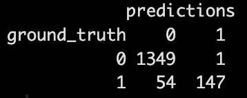
In this example:

• The top-left value is the number of true positives, being the number of instances correctly classified as not spam in the test data
• The top-right is the number of false negatives, or those instances incorrectly classified as spam
• The bottom-left is the number of false positives, the spam data samples erroneously classified as not spam
• The bottom-right is the number of true negatives, which are those instances of spam correctly classified as spam.

Given true positives and true negatives collectively outnumber false predictions in this confusion matrix, the classifier appears to perform well. As mentioned, however, this confusion matrix displays the actual number of correct and incorrect predictions for each class. What if we instead want to see each classes’ percentage of correct and incorrect predictions?

Step 5. Compute evaluation metrics

The confusion matrix provides a readily accessible visualization of classifier predictive results. As such, it can be useful for calculating an array of classifier model evaluation metrics. In fact, the confusionMatrix() function in R's cavet package produces both a confusion matrix and summary report of widely used metrics for gauging model performance.

# convert lists into data frame format
data <- data.frame(ground_truth = ground_truth, predictions = predictions)
# create confusion matrix with caret package's confusionMatrix
cm <- confusionMatrix(as.factor(data$predictions), as.factor(data$ground_truth))

print(cm)

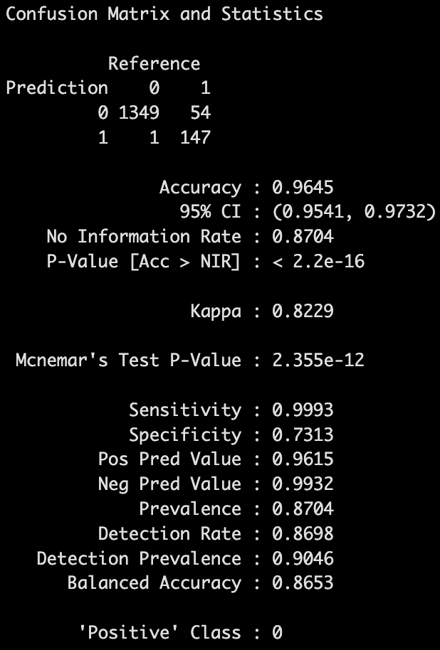
The first value listed beneath the confusion matrix is accuracy. This is perhaps the most basic evaluation metric for classification models, although it does not always offer a complete of model performance. Imagine we run a classifier on a data set of 100 instances. The model’s confusion matrix shows only one false negative and no false positives. For our spam filtering task, this accuracy of 99% is desirable. But, what if our model aims to classify highly contagious diseases? That 1% misclassification poses an enormous risk. Thus, other evaluation metrics can be used to provide a better picture of the performance of a classification algorithm.

Some of the most widely used evaluation metrics, however, are in the penulimate and largest block returned in the report. Here is a rundown of perhaps the most widely adopte metrics from that report:

• Sensitivity — A conditional metric also known as true positive rate (TPR) or recall. It indicates the proportion of positive predictions for a given class out of all actual instances of that class.

• Specificity — A conditional metric also known as true negative rate (TNR). It is the proportion of correct negative predictions out of actual non-instances of a given class.

• Pos Pred Value (PPV) — An unconditional metric more popularly known as precision. It indicate the likelihood that a chosen instance actually belongs to a specified class.

• Neg Pred Value (NPV) — An unconditional metric that signifies probability a chosen instance will not belong to a given class.

Many of other values provided in this report are perhaps less well-known. Nevertheless, here is a quick overview of their meaning:

• No Information Rate (NIR) — This indicates the project accuracy if the model classified every data sample as "True," in our case "Not Spam."

• P-Value — This is a measurement that compares the model's accuracy to its NIR. In general, a smaller p-value indicates better model performance.

• Kappa — Also called Cohen's kappa. This is another accuracy metric that indiciates the level of agreement between a the ground truth and predictions beyond the level fo agreement resulting from chance. Although Kappa can reach as far as -1, it typically ranges between 0 and 1. 0 indicates the model's accuracy is no better than random chance, and 1 indicates there is perfect agreement between model predictions and actual values not attributable to chance.

• Mcnemar's Test P-Value — A statistical measurement of the p-value comparing false negatives to false positives. In general, a p-value smaller than .05 here means the difference between false negatives and false positives is statistically significant.

• Detection Rate — The proportion of true positives that the model correctly classifies. This is the number of true positives divided by the total actual observations.

• Detection Prevalence — The proportion of positive cases the model classifies. In other words, the sum of true positives and false positives divided by total actual observations.

Step 6. Visualize confusion matrix

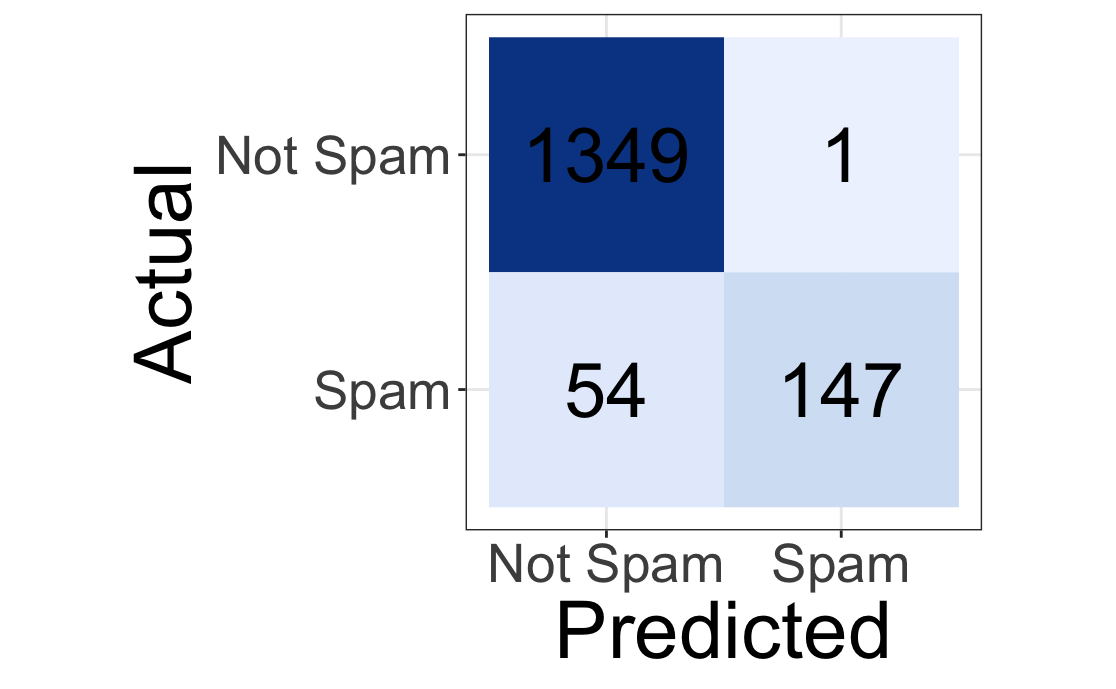
Using print() with R's confusionMatrix() and table() functions command provides a basic confusion matrix for rudimentary model evaluation. But in some cases, one may want a more robust confusion matrix with labels. R's various packages provides several approaches for completing this task. One option is to create a heatmap using the ggplot2 package. Here is the code for visualizing our confusion matrix with that package:

# create new confusion matrix for Actual + Predicted labels
con_matrx <- table(Actual = ground_truth, Predicted = predictions)

# convert new confusion matrix to data frame
hm <- as.data.frame(as.table(con_matrx))

# create confusion matrix with ggplot2
ggplot(hm, aes(x = Predicted, y = Actual, fill = Freq)) +
  geom_tile() + theme_bw() + coord_equal() +
  scale_fill_distiller(palette = "Blues", direction = 1) +
  guides(fill = FALSE) +
  geom_text(aes(label = Freq), color = "black", size = 10) +
  # following lines only increase text size (optional)
  theme(axis.text.x = element_text(size = 20),
      axis.text.y = element_text(size = 20),
      axis.title.x = element_text(size = 30),
      axis.title.y = element_text(size = 30))

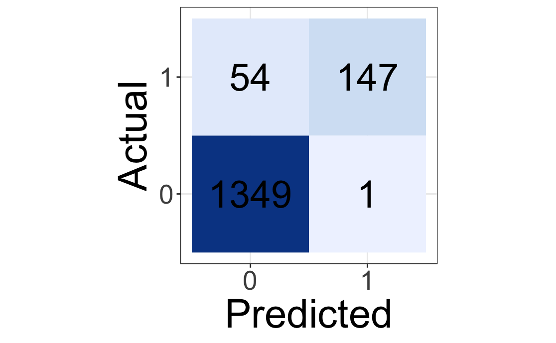
Comparing the heatmap to our earlier, rudimentary matrices, users may notice that the quadrant arrangmenets vary between them. Whereas the total number of true positives were earlier listed in the upper-left quadrant, they appear in the lower-left quadrant of our heatmap. While this different arrangement is not necessarily a problem, many confusion matrices for binary classification in literature list true positives in the upper-left and true negatives in the lower-right. We can manually rearrange the heatmap tiles to match this convention using the scale_x_discrete() and scale_y_discrete() functions. These functions allow us to specificy which rows and columns corresond to which values. Remember that 0 denotes Not Spam and 1 denotes Spam:

# create new confusion matrix for Actual + Predicted labels
con_matrx <- table(Actual = ground_truth, Predicted = predictions)

# convert confusion matrix to data frame
hm <- as.data.frame(as.table(con_matrx))

# same code as previous block
plot <- ggplot(hm, aes(x = Predicted, y = Actual, fill = Freq)) +
  geom_tile() + theme_bw() + coord_equal() +
  scale_fill_distiller(palette = "Blues", direction = 1) +
  guides(fill = FALSE) +
  geom_text(aes(label = Freq), color = "black", size = 10)

# reorder quadrants
plot +
  scale_x_discrete(limits = c("0", "1"),
                    labels = c("Not Spam", "Spam")) +
  scale_y_discrete(limits = c("1", "0"),
                    labels = c("Spam", "Not Spam")) +
  # following lines only increase text size (optional)
  theme(axis.text.x = element_text(size = 20),
        axis.text.y = element_text(size = 20),
        axis.title.x = element_text(size = 30),
        axis.title.y = element_text(size = 30))

R allows for another readily implemented confusion matrix visualization method using the ConfusionTableR package:

# create confusion matrix with ConfusionTableR pkg
binary_visualiseR(
  train_labels = as.factor(data$predictions),
  truth_labels = as.factor(data$ground_truth),
  class_label1 = "Not Spam",
  class_label2 = "Spam",
  quadrant_col1 = "#0672FF",
  quadrant_col2 = "#4CC9F0",
  text_col = "white"
)

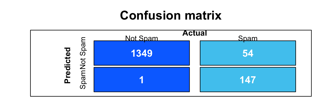
As with out initial heatmap matrix, the quadrants in the ConfusionTableR method diverge from our initial, more rudimentary matrices. Specifically, the false positive and false negative quadrants are interchanged, although all of our quadrant values remain correct. Unlike the heatmap matrix, ConfusionTableR does not allow for customizing the quadrant arrangement nor modifying the size of our matrix's text labels. But it does display the matrix alongside common evaluation metrics, such as precision and recall.

Summary and next steps

This beginner tutorial provides an overview for how to use a number of packages to create a confusion matrix and compute common evaluation metrics in R for a simple binary classification problem. The functions used in this tutorial can also create confusion matrices for multi-class classification problems. There are, in fact, a number of other evaluation visualizations, such as ROC curve and AUC, for measuring the quality of classification models.

Try watsonx for free

Build an AI strategy for your business on one collaborative AI and data platform called IBM watsonx, which brings together new generative AI capabilities, powered by foundation models, and traditional machine learning into a powerful platform spanning the AI lifecycle. With watsonx.ai, you can train, validate, tune, and deploy models with ease and build AI applications in a fraction of the time with a fraction of the data.

Try watsonx.ai, the next-generation studio for AI builders.

Next steps

Explore more articles and tutorials about watsonx on IBM Developer.

Also, to learn more about classification or regression algorithms using Python and scikit-learn, see these tutorials in the Getting started with machine learning learning path:

• Tutorial: Learn classification algorithms using Python and scikit-learn