Using random forest to predict credit defaults using Python

Random forest is a machine learning algorithm that combines the output from multiple decision trees to get a single result. Just like decision trees, random forest models can be used for both classification and regression tasks.

The basic idea behind decision trees is to start with a basic question and split the data into decision nodes with the final decision denoted by a leaf node. Random forests are an ensemble of decision trees, which helps to overcome decision tree limitations, such as bias and overfitting.

By default, the random forest algorithm uses bootstrapping to sample the data for building individual decision trees. Bootstrapping is when a subset of data is randomly selected from the full data set. Some data points are duplicated to bring the size of the subset of data to the same size as the original data set. This is partly how the different decision trees can arrive at different results.

Multiple hyperparameters can be used to fine-tune decision trees, such as node size, number of trees, and number of features sampled. For regression tasks, the random forest algorithm will average the decision tree results. For classification tasks, the random forest classifier will take a majority vote. Like decision trees, one of the big advantages of a random forest is interpretability using feature importance.

For a more detailed description, see What is random forest?.

In this tutorial, you'll use scikit-learn to apply random forest classification to predict credit card defaults.

Prerequisites

To follow this tutorial, you must:

• Create an IBM Cloud account so that you can create a watsonx.ai project.

• Install scikit-learn

Steps

Step 1. Set up your environment

While you can choose from several tools, this tutorial walks you through how to set up an IBM account to use a Jupyter Notebook. Jupyter Notebooks are widely used within data science to combine code, text, images, and data visualizations to formulate a well-formed analysis.

1. Log in to watsonx.ai using your IBM Cloud account.

2. Create a watsonx.ai project.

3. Create a Jupyter Notebook.

From here, a notebook environment opens for you to load your data set and copy code from this beginner tutorial to tackle a simple classification problem using a random forest classifier.

Note that the initial exploratory steps are very similar to those you would take for any machine learning classification problem, such as using SVM as described in this Python tutorial and this R tutorial.

Step 2. Import libraries and load the data set

First, we'll import commonly used data processing and manipulation libraries. We'll also import the libraries required for creating a random forest model. If the necessary libraries are not installed, you can resolve this by using the pip install command directly in the notebook using a code cell.

!pip3 install sklearn
!pip3 install xlrd

Remember to restart the notebook after installing the library.

The task for this tutorial will be to predict the probability of a customer defaulting on a loan. The target variable is "default payment" (Yes=1; No=1). Details of the data measurements can be found in UCI's data repository.

#Load the required libraries
import pandas as pd
import numpy as np
import seaborn as sns
from sklearn.utils import resample
from sklearn.model_selection import train_test_split
from sklearn.svm import SVC
from sklearn.metrics import confusion_matrix
from sklearn.ensemble import RandomForestClassifier
import matplotlib.colors as colors
import matplotlib.pyplot as plt


# Import the data set
df = pd.read_excel('https://archive.ics.uci.edu/ml/machine-learning-databases/00350/default%20of%20credit%20card%20clients.xls', header=1)

Step 3: Explore the data set

Exploring the data set is a critical step that should not be overlooked. This can help you to understand what data is available and the quality of that data. This will guide both data cleaning and modeling decisions. First, let's look at the first 10 rows of the data frame.

#Explore the first ten rows of the data set
df.head(10)

Each row represents an individual. Some columns that could be useful are credit limit, prior payment status, bill and payment amounts, and our target variable that indicates default next month.

# Rename the columns
df.rename({'default payment next month': 'DEFAULT'}, axis='columns', inplace=True)

#Remove the ID column as it is not informative
df.drop('ID', axis=1, inplace=True)
df.head()

The code above renames the default column to something a bit shorter. We also drop the ID column, because it doesn't contain any information relevant to the analysis.

Step 4: Analyze missing data

One key step is to check for null values or other invalid input that will cause the model to throw an error. This is where referencing the data dictionary will be useful, so you know what is valid for a given data set.

# check dimensions for invalid values
print(df['SEX'].unique())
print(df['MARRIAGE'].unique())
print(df['EDUCATION'].unique())
print(df['AGE'].unique())

# count missing or null values
print(len(df[pd.isnull(df.SEX)]))
print(len(df[pd.isnull(df.MARRIAGE)]))
print(len(df[pd.isnull(df.EDUCATION)]))
print(len(df[pd.isnull(df.AGE)]))

#count of missing data
len(df.loc[(df['EDUCATION'] == 0) | (df['MARRIAGE'] == 0)]) #output: 68

The output indicates that some of the data does not align with the data definitions, specifically EDUCATION and MARRIAGE columns. EDUCATION includes three types of invalid values, which are 0, 5, and 6 and MARRIAGE includes 0 as an invalid value. We'll assume that a 0 encoding is supposed to represent missing data and that a value of 5 or 6 within EDUCATION is representative of other unspecified education levels (for example, Ph.D. or a Master's degree), which is not represented within the data definition.

68 rows exist in the DataFrame where either the EDUCATION or the MARRIAGE column is zero. Next, let's filter the rows where the EDUCATION and MARRIAGE columns have non-zero values.

#Filter the DataFrame
df_no_missing_data = df.loc[(df['EDUCATION'] != 0) & (df['MARRIAGE'] != 0)]
df_no_missing_data.shape

The code above creates a new DataFrame with the missing values for EDUCATION and MARRIAGE removed. We end up with 29,932 rows remaining.

The next step is to check whether the target variable, whether or not someone defaulted, is balanced.

# Explore distribution of data set
# count plot on ouput variable
ax = sns.countplot(x = df_no_missing_data['DEFAULT'], palette = 'rocket')

#add data labels
ax.bar_label(ax.containers[0])

# add plot title
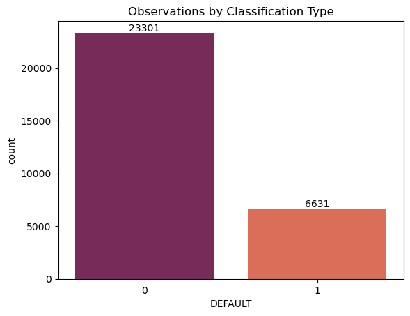
plt.title("Observations by Classification Type")

# show plot
plt.show()

The following chart shows counts of people who have defaulted (1) and haven't defaulted (0). Unsurprisingly, most people have not defaulted on their loans. To address this class imbalance, we will need to down sample the data.

Step 5: Downsample the data set

The first step in downsampling is to split the data based on those who defaulted on their loan and those who did not default on their loan. For the purposes of this tutorial, we will then randomly select 1,000 samples from each category. In practice, a better method is to make sure the sample is balanced across all potentially biased variables, such as SEX, AGE, and MARRIAGE status. The two data sets will then be merged back together to create an analysis data set.

from sklearn.utils import resample

# split data
df_no_default = df_no_missing_data.loc[(df_no_missing_data['DEFAULT']==0)]
df_default = df_no_missing_data.loc[(df_no_missing_data['DEFAULT']==1)]

# downsample the data set
df_no_default_downsampled = resample(df_no_default, replace=False, n_samples=1000, random_state=42 )
df_default_downsampled = resample(df_default, replace=False, n_samples=1000, random_state=42 )

#check ouput
len(df_no_default_downsampled)
len(df_default_downsampled)

# merge the data sets
df_downsample = pd.concat([df_no_default_downsampled, df_default_downsampled ])
df_downsample.shape

Step 6: Hot encode the independent variables

The modeling library that we used in this tutorial, scikit-learn, does not support categorical data. The solution is to convert each category into a binary variable with a value of 0 or 1. Once this change is made, the model should not treat the data as continuous. Pandas has a very convenient function to do just this, called get_dummies.

One thing to keep in mind when creating models is to avoid bias. One very important way to do this is to not use variables associated with protected attributes as independent variables. In this case, SEX, AGE, and MARRIAGE clearly fall into that category. EDUCATION is somewhat more ambiguous. Since it is not critical for the purposes of this tutorial, we will drop that as well.

# isolate independent variables
X = df_downsample.drop(['DEFAULT','SEX', 'EDUCATION', 'MARRIAGE','AGE'], axis=1).copy()

X_encoded = pd.get_dummies(data=X, columns=['PAY_0', 'PAY_2', 'PAY_3', 'PAY_4', 'PAY_5', 'PAY_6'])
X_encoded.head()

It is generally a good idea to normalize your data, although how important this is can differ based on the algorithm used and the problem to be solved. When it comes to using random forest models on classification tasks, like the one presented here, the general consensus is normalization is not necessary. However, classification can be impacted How data normalization affects your random forest algorithm. Because the problem in this tutorial is classification, we will move on to the next step.

Step 8: Split the data set

Splitting the data into test and training sets is critical for understanding how your model will perform on new data. The random forest model uses the training data set to learn what factors should become decision nodes. The test set helps us evaluate how often those decisions lead to the correct decision.

from sklearn.preprocessing import scale
y = df_downsample['DEFAULT'].copy()
X_train, X_test, y_train, y_test = train_test_split(X_encoded, y, test_size=0.3, random_state=42)

Step 9: Classify accounts and evaluate the model

Now its time to build an initial random forest model by fitting it using the training data and evaluating the resulting model using the test data. To make that evaluation easier, we'll plot the results using a confusion matrix.

from sklearn.metrics import confusion_matrix
from sklearn.metrics import ConfusionMatrixDisplay
from sklearn.metrics import accuracy_score

clf_rf = RandomForestClassifier(max_depth=2, random_state=0)
clf_rf.fit(X_train, y_train)

#calculate overall accuracy
y_pred = clf_rf.predict(X_test)
accuracy = accuracy_score(y_test, y_pred)
print(f'Accuracy: {accuracy:.2%}')

class_names = ['Did Not Default', 'Defaulted']
disp = ConfusionMatrixDisplay.from_estimator(
        clf_rf,
        X_test,
        y_test,
        display_labels=class_names,
        cmap=plt.cm.Blues)

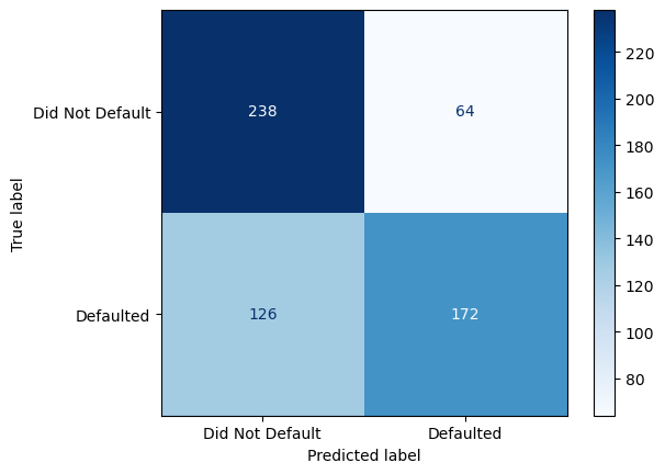
As we can see, the model performance could be improved. Of the 302 accounts that did not default, only 79% were correctly predicted. Of the 298 accounts that did default, only 58% were correctly predicted.

Step 10: Optimize the model with hyperparameter tuning

Cross validation and GridSearchCV are useful tools for finding the best hyperparameters for models. When it comes to random forest models, we'll focus on max_depth, min_samples_split, min_samples_leaf, and max_leaf_nodes. Here's a quick overview of what those hyperparameters mean:

• max_depth: the maximum number levels the decision trees that make up the random forest are allowed to have
• min_samples_split: the minimum number of samples that must be in a node for a decision split to be allowed
• min_samples_leaf: the minimum number of samples that must exist in a leaf node

Larger numbers on min_samples_split and min_samples_leaf, and smaller numbers on max_depth help, helps avoid overfitting.

Another commonly used hyperparameter is max_features. This is the number of features that the model will try out when attempting to create a decision node. The n_estimators hyperparameter controls the number of decision trees that are created as part of the random forest model. For more details and other hyperparameters that can be tuned, see the sklearn random forest documentation.

from sklearn.model_selection import RandomizedSearchCV

param_grid = {
    'max_depth':[2,3,4,5],
    'min_samples_split':[2,3,4,5],
    'min_samples_leaf':[2,3,4,5]
}
rf_random = RandomizedSearchCV(
    estimator = clf_rf, param_distributions = param_grid, 
    n_iter = 100, cv = 3, verbose=2, random_state=42, n_jobs = -1)

# Fit the random search model
rf_random.fit(X_train, y_train)
rf_random.best_params_

# refit model with optimal hyperparameters
clf_rf = RandomForestClassifier(
    max_depth=5, min_samples_split=5, min_samples_leaf=2,
    random_state=0)
clf_rf.fit(X_train, y_train)

#calculate overall accuracy
y_pred = clf_rf.predict(X_test)
accuracy = accuracy_score(y_test, y_pred)
print(f'Accuracy: {accuracy:.2%}')

# plot confusion matrix
class_names = ['Did Not Default', 'Defaulted']
disp = ConfusionMatrixDisplay.from_estimator(
        clf_rf,
        X_test,
        y_test,
        display_labels=class_names,
        cmap=plt.cm.Blues)

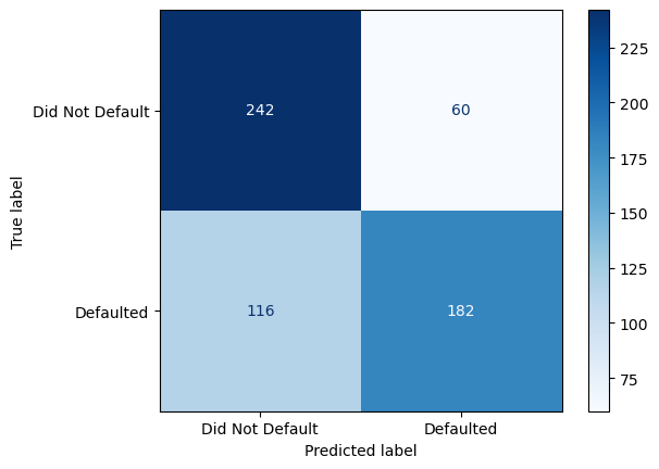
Just by trying a few different hyperparameters, we've improve the accuracy by just over 2%. This may not seem like much, but in some applications that can make all the difference. Some ways to improve the predictions are to extend the ranges of the hyperparameters where we hit the max and to explore other hyperparameters. Another option is to use Principal Component Analysis (PCA), which you can learn about in this Python tutorial.

Summary

In this tutorial, you learned how to apply random forest classification to predict credit card defaults. You also fine tuned your classifier model by optimizing the hyperparameters, which resulted in a small improvement in accuracy.

Try watsonx for free

Build an artificial intelligence (AI) strategy for your business on one collaborative AI and data platform called IBM watsonx, which combines new generative AI capabilities powered by foundation models and traditional machine learning into a powerful platform spanning the AI lifecycle. With watsonx.ai, you can train, validate, tune, and deploy models with ease and build AI applications in a fraction of the time with a fraction of the data.

Try watsonx.ai, the next-generation studio for AI builders.

Next steps

Explore more articles and tutorials about watsonx on IBM Developer.

Also, to learn more about other supervised learning algorithms that you can apply to classification and regression problems, see these tutorials in the Getting started with machine learning learning path:

• Tutorial: Learn classification algorithms using Python and scikit-learn
• Tutorial: Learn regression algorithms using Python and scikit-learn