Reducing dimensionality with principal component analysis with Python

Principal component analysis (PCA) is a linear dimensionality reduction technique that transforms potentially correlated variables into a smaller set of variables called principal components. PCA reduces the number of dimensions while retaining the most information from the original data set.

PCA is an unsupervised learning algorithm that is commonly used by data scientists for data preprocessing. It transforms a large data set into a lower dimensional space, extracting the most informative features while preserving the most relevant information from the initial data set. This data preprocessing reduces model complexity as the addition of each new feature negatively impacts model performance, which is also commonly referred to as the “curse of dimensionality.”

By projecting high-dimensional data into a smaller feature space, PCA also minimizes, or altogether eliminates, common issues such as multicollinearity and overfitting. Multicollinearity occurs when two or more independent variables are highly correlated with one another, which is problematic for causal modeling. Overfit models will also generalize poorly to new data, diminishing their value altogether.

This simplification of data also has implications for data visualization tasks and its additional use with other machine learning algorithms, like linear or logistic regression algorithms. Data in a lower-dimensional space both improves the interpretability of data visualizations and overall model performance.

While there are other variations of PCA, such as principal component regression and kernel PCA, this tutorial focuses on the primary method of PCA.

In this tutorial, you use Python to apply PCA on a popular wine data set to demonstrate how to reduce dimensionality within the data set. Each wine sample in the data set is categorized into one of three classes (class 0, class 1, and class 2), which indicates the grape's origin. The goal is to optimize the classification of these wine classes using PCA. For more information on this data set, refer to the documentation on the UCI ML repository where scikit-learn sourced this data.

Prerequisites

To follow this tutorial, you must:

• Create an IBM Cloud account

• Install scikit-learn

If you want to execute these instructions without the need to download, install, and configure tools, you can use the hands-on guided project, Practice using PCA to reduce dimensionality.

Steps

Step 1. Set up your environment

While you can choose from several tools, this tutorial walks you through how to set up an IBM account to use a Jupyter Notebook. Jupyter Notebooks are widely used within data science to combine code, text, images, and data visualizations to formulate a well-formed analysis.

1. Log in to watsonx.ai using your IBM Cloud account.

2. Create a watsonx.ai project.

3. Create a Jupyter Notebook.

From here, a notebook environment opens for you to load your data set and copy code from this beginner tutorial to tackle a dimensionality reduction problem.

Step 2. Import libraries and load the data set

You must import the necessary Python libraries, Pandas, and Matplotlib, to work with the wine data set. This helps you to conduct an exploratory data analysis for any relevant data manipulation and data visualization to prepare the data for machine learning tasks. If any libraries are not installed, you can resolve this with a quick pip install.

This data is based on an analysis of wines that are grown in Italy from three different cultivars. Thirteen features were found in each of the three types of wines to help distinguish them from one another.

# Load the required libraries
import numpy as np
import pandas as pd
import matplotlib.pyplot as plt
import seaborn as sns
from sklearn.model_selection import train_test_split
from sklearn.preprocessing import StandardScaler
from sklearn.decomposition import PCA
from sklearn.datasets import load_wine
from sklearn.model_selection import train_test_split

# Load the Wine Quality data set

data = load_wine()
df = pd.DataFrame(data.data, columns=data.feature_names)
df['target'] = pd.Series(data.target)
X = df.iloc[: ,:13]
y = df['target']

column_names = df.columns
column_names = column_names.to_list()

Step 3. Explore the data set

Before initiating data preprocessing, you should conduct an exploratory data analysis to understand the data's structure and format, including the types of variables, their distributions, and the overall organization of information. This helps you determine whether PCA is necessary to model the data.

You can start by understanding the shape of the data set, which lets you see that you have a 13-dimensional data set. You can explore further to see whether any of the features are correlated to one another, which indicates a potential need for dimensionality reduction.

df.shape

Some visualizations that you might want to use to explore the data include pair plots, histograms, and correlation heatmaps. Because this is a higher dimensional data set, some visualizations are more effective than others at highlighting correlations between variables.

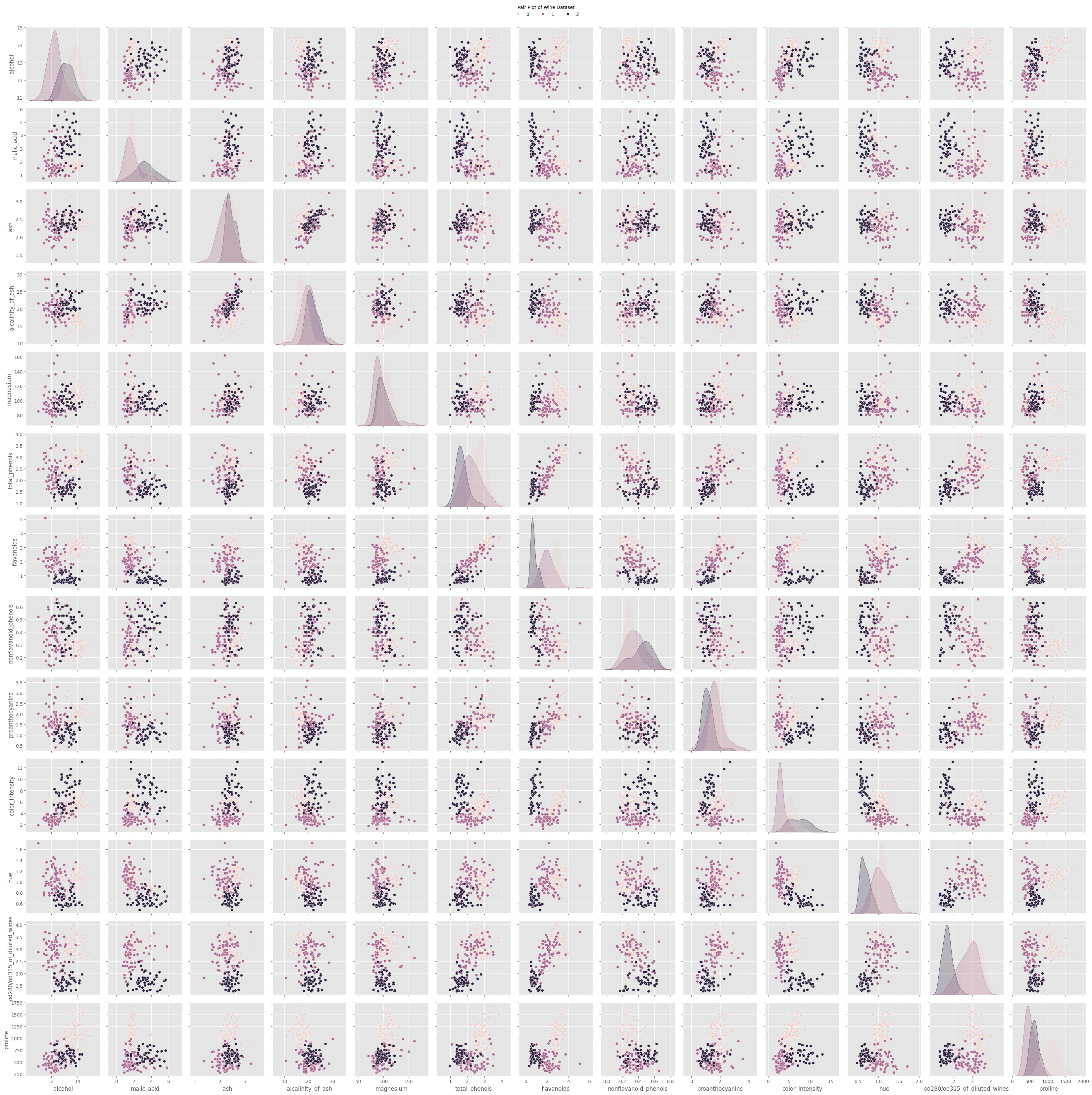
Pair plots

Given the number of dimensions in this data set, pair plots might not be the most effective visualization to identify correlations between data.

ax = sns.pairplot(df, hue='target')
sns.move_legend(
    ax, "lower center",
    bbox_to_anchor=(.5, 1), ncol=3, title="Pair Plot of Wine             Dataset", frameon=False)

plt.tight_layout()
plt.show()

While you can see distributions and the direction of any correlation between classes by feature, it can be hard to read the data labels without zooming in, making the interpretation of the visualization more difficult.

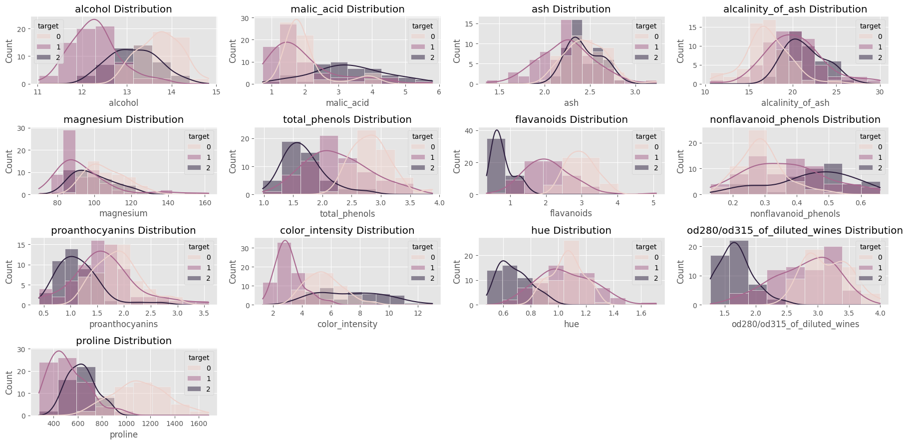
Histograms

Histograms show you the distributions of the different features for each category of wine.

# Visualize the distribution of each feature using histograms.
plt.figure(figsize=(18, 9))
for i, feature in enumerate(column_names[:-1]):
    plt.subplot(4, 4, i + 1)
    sns.histplot(data=df, x=feature, hue='target', kde=True)
    plt.title(f'{feature} Distribution')
plt.tight_layout()
plt.show()

Here, you can see a similar distribution of data by type for the following features: ash, alkalinity of ash, and magnesium.

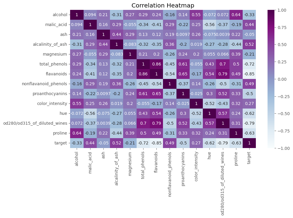
Correlation heatmaps

Correlation heatmaps might be the most helpful in identifying positive and negative correlations between attributes.

# Note issue with older version of seaborn: https://github.com/mwaskom/seaborn/issues/3478

corr = df.corr()
plt.figure(figsize=(10,6))
sns.heatmap(corr,
            xticklabels=corr.columns.values,
            yticklabels=corr.columns.values,
            cmap="BuPu",
            vmin=-1,
            vmax=1,
            annot=True)
plt.title("Correlation Heatmap")
plt.show()

Darker cells indicate positive correlation whereas light gray/white cells signal negative correlation between features. For example, you can see a high positive correlation between flavonoids and total phenols at 86%.

Step 4. Split the data set

Given the exploratory analysis, you can conclude that there are some correlated features within the data set, and that the model might benefit from PCA to reduce the number of dimensions in the data.

From here, you split the data set into two sets, a training set and the test set.

X_train, X_test, y_train, y_test = train_test_split(X, y, test_size=0.2, random_state=0)

Step 5. Standardize data points through feature scaling

Next, you standardize the data by scaling and centering it to have a mean of zero and a standard deviation of one. This is a common practice when implementing PCA because this approach is affected by variables with different scales. Without this standardization, PCA might place more weight to variables with larger scales, incorrectly attributing more importance to them. To read more on the importance of feature scaling, explore the scikit-learn documentation.

#scaling and centering the data
sc = StandardScaler()
X_train_scaled = sc.fit_transform(X_train)
X_test_scaled = sc.transform(X_test)

Step 6. Determine the optimal value for the n_components parameter

There are a few different ways that you can determine the ideal value for the n_components parameter to apply PCA effectively. Through two popular data visualizations, you can identify the optimal number of principal components to capture the most information from the original data set.

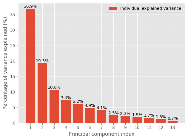
The first data visualization is a plot of the explained variance percentage of individual components and the percentage of total variance that is captured by all principal components.

# calculate covariance matrix, eigenvalues and eigenvectors
cov_mat = np.cov(X_train_scaled.T)
eigen_vals, eigen_vecs = np.linalg.eig(cov_mat)

exp_var = []

# Sort the eigenvalues in descending order
eigen_vals = np.sort(eigen_vals)[::-1]

for i in eigen_vals:
  var = (i / np.sum(eigen_vals)) * 100
  exp_var.append(var)

bar = plt.bar(range(1, 14), exp_var, align='center',
        label='Individual explained variance')

# Adding data labels to the top of bars 
for i, bar in enumerate(bar):
    plt.text(bar.get_x() + bar.get_width() / 2, bar.get_height(), f'{exp_var[i]:.1f}%', 
             ha='center', va='bottom')

plt.ylabel('Percentage of variance explained (%)')
plt.xlabel('Principal component index')
plt.xticks(ticks=list(range(1, 14)))
plt.legend(loc='best')
plt.tight_layout()

Here, you're looking for the number of components that explain most of the variance in the data. You might want to choose the number of components that explain 80-90% of the variation to ensure that you're capturing the most information from the initial data set. By choosing five components, 83.6% of the variance would be explained from the initial data set.

The second data visualization is a scree plot.

# generate scree plot
pca = PCA()
X_train = pca.fit_transform(X_train_scaled)
explained_variance = pca.explained_variance_ratio_
plt.plot(pca.explained_variance_, marker='o')
plt.xlabel("Eigenvalue number")
plt.ylabel("Eigenvalue size")
plt.title("Scree Plot")

Here, you're looking for the point at which the line "elbows." The visualization here suggests that two or three principal components might be ideal.

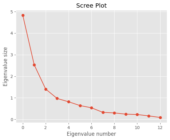
Through some visual inspection of these two plots, you'll use two principal components, but through trial and error, you can test which number of components yields the best results as well.

Step 7. Apply PCA to the scaled training data

Now that you know the subset of components that you'll select, you can proceed with applying PCA to the data set. In this step, you are applying an orthogonal transformation to create a linear combination of the features from the original data set. While you could incorporate more principal components, two principal components capture most (56.2%) of the variance in the data set. Because this isn't the ideal 80-90% of variation that you typically look for, it's worth noting that you lose some information from the original data set.

pca = PCA(n_components=2)
principalComponents = pca.fit_transform(X_train_scaled)
pca_df = pd.DataFrame(data = principalComponents
             , columns = ['principal component 1', 'principal component 2'])

pca_df.reset_index(drop=True, inplace=True)
y_train.reset_index(drop=True, inplace=True)
y_train = pd.DataFrame(y_train)
final_pca_df = pca_df
final_pca_df['target'] = y_train

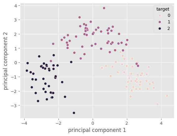
Step 8. Visualize the output

You use a scatter plot to plot and visualize the principal components, which provides a 2-dimensional view of the original 13-dimensional data set.

ax = sns.scatterplot(x =final_pca_df.iloc[:,0], y = final_pca_df.iloc[:,1],
hue = 'target',
data=final_pca_df,
legend=True)
plt.show()

Here, you can also observe the class separation between the different types of wine in the data set within the projected data.

Summary and next steps

In this tutorial, you learned how to apply PCA to reduce the dimensionality of a 13-dimensional wine data set. In future tutorials, you'll apply this technique to visualize high-dimensional data as well as to optimize performance.

Try watsonx for free

Build an artificial intelligence (AI) strategy for your business on one collaborative AI and data platform called IBM watsonx, which combines new generative AI capabilities powered by foundation models and traditional machine learning into a powerful platform spanning the AI lifecycle. With watsonx.ai, you can train, validate, tune, and deploy models with ease and build AI applications in a fraction of the time with a fraction of the data.

Try watsonx.ai, the next-generation studio for AI builders.

Next steps

Explore more articles and tutorials about watsonx on IBM Developer.

Also, to learn more about other supervised learning algorithms that you can apply to classification and regression problems, see these tutorials in the Getting started with machine learning learning path:

• Tutorial: Learn classification algorithms using Python and scikit-learn
• Tutorial: Learn regression algorithms using Python and scikit-learn